from tqdm.notebook import trange
import numpy as np
import matplotlib.pyplot as plt
from sklearn.linear_model import LinearRegression

import torch
from torch import nn
from torch.utils.data import Dataset, DataLoader

plt.rcParams['figure.figsize'] = (11, 7)
plt.rcParams['font.size'] = 20
plt.rcParams['lines.linewidth'] = 3.006 Basics of Neural Networks
Disclaimer
- Seminar is very introductory
- No deep theory
- Basic examples of main parts
Ther are a lot of libraries to do deep learning in Python (Pytorch, TesnorFlow, JAX). You may even do it with pure numpy. And even in Java or C++.
In this example we will use PyTorch.
Multilayer Perceptron
First idea of Neural Networks by Frank Rosenblatt, 1958.
First appearance of ubiqutous and famous convolutional neural network (whatever it is) apper also in 1950s. Formalized in 1990.
Now neural networks (expecially large language models) are among most hot topics in the web.

What is this anyway?
Lets start with linear regression
Function we wish to approximate: \(y_{true} = f^*(x)\)
Machine learning model: \(\hat{y} = f(x)\, , \, \hat{y} \approx y_{true}\)
And if we use simple linear regression (with single feature):
\[y = a x + b\]
x = np.linspace(0, 50, 20)
noise = np.random.normal(0, 1.2, size=20) * 10
y_true = 5 * x - 53
y_noisy = (5 * x - 53) + noise

plt.plot(x, y_true, 'r', label='Real function')
plt.plot(x, y_noisy, 'o', c='b', label='Noisy observations')

plt.xlabel("x", fontsize=15)
plt.ylabel('y', fontsize=15)
plt.legend();
lin_reg = LinearRegression(fit_intercept=True)
lin_reg.fit(x.reshape(-1, 1), y_noisy)
plt.plot(x, lin_reg.predict(x.reshape(-1, 1)), '--', c='g', label="ML model")
plt.plot(x, y_true, 'r', label='Real function')
plt.plot(x, y_noisy, 'o', c='b', label='Noisy observations')
plt.xlabel("x", fontsize=15)
plt.ylabel('y', fontsize=15)
plt.legend();Now say we have \(n\) features:
\[y = a_1 \cdot x_1 + a_2 \cdot x_2 + \dots + a_n \cdot x_n + b \, ,\]
and in vector form:
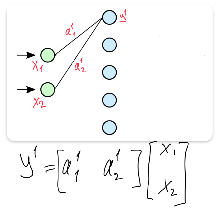
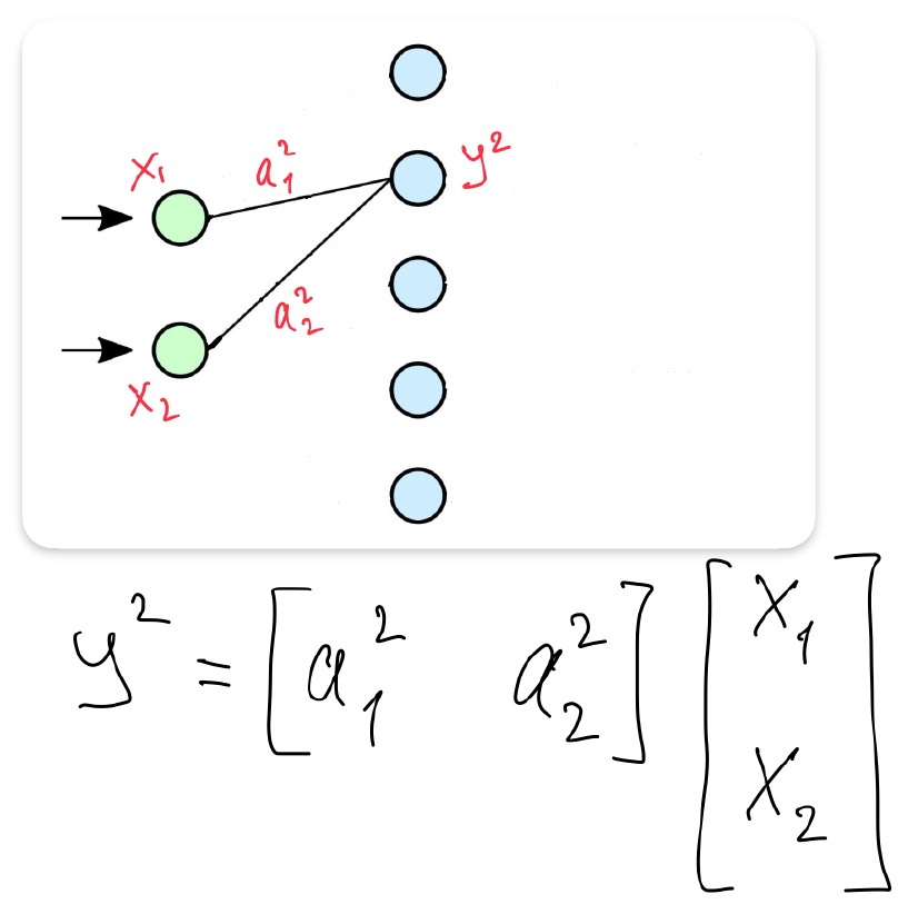
\[y = \begin{bmatrix} a_1 & a_2 & \cdots & a_n \end{bmatrix} \begin{bmatrix} x_1 \\ x_2 \\ \vdots \\ x_n \end{bmatrix} + b \, .\] ### Not single ouput?
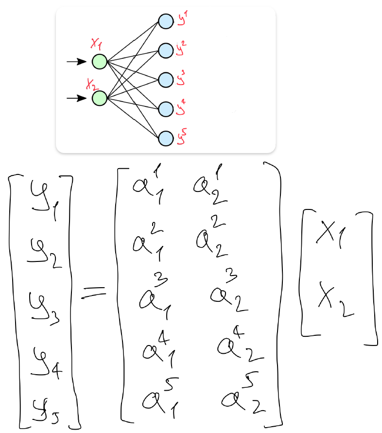
You may want to predict multiple outputs with your model (say, not only the price of a house, but also the income of a real estate agent). Sklearn in this case will fit two separate models simultaneously:
\[ \begin{cases} y^1 & = & a_1^1 \cdot x_1 + a_2^1 \cdot x_2 + \dots + a_n^1 \cdot x_n + b^1 \\ y^2 & = & a_1^2 \cdot x_1 + a_2^2 \cdot x_2 + \dots + a_n^2 \cdot x_n + b^2 \end{cases} \, , \]
with \(k\) targets:
\[ \begin{cases} y^1 & = & a_1^1 \cdot x_1 + a_2^1 \cdot x_2 + \dots + a_n^1 \cdot x_n + b^1 \\ y^2 & = & a_1^2 \cdot x_1 + a_2^2 \cdot x_2 + \dots + a_n^2 \cdot x_n + b^2 \\ & \cdots & \\ y^k & = & a_1^k \cdot x_1 + a_2^k \cdot x_2 + \dots + a_n^k \cdot x_n + b^k \end{cases} \, , \]
and in matrix form
\[ \begin{bmatrix} y_1 \\ y_2 \\ \vdots \\ y_k \end{bmatrix} = \begin{bmatrix} a_1^1 & a_2^1 & \cdots & a_n^1 \\ a_1^2 & a_2^2 & \cdots & a_n^2 \\ \vdots & \vdots & \ddots & \vdots \\ a_1^k & a_2^k & \cdots & a_n^k \\ \end{bmatrix} \begin{bmatrix} x_1 \\ x_2 \\ \vdots \\ x_n \end{bmatrix} + \begin{bmatrix} b_1 \\ b_2 \\ \vdots \\ b_k \end{bmatrix} \, , \]
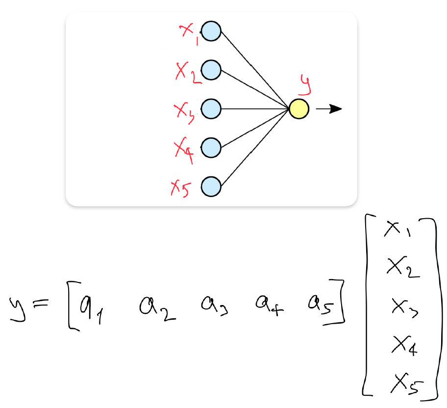
Even shorter with matrix form:
\[y = Ax + b \, ,\]
where \(y \in \mathbb{R}^k\), \(x \in \mathbb{R}^n\), and \(b \in \mathbb{R}^k\) are vectors. \(A \in \mathbb{R}^{k \times n}\) is a matrix.
It’s time to introduce multilayer perceptron!
Two layer MLP:
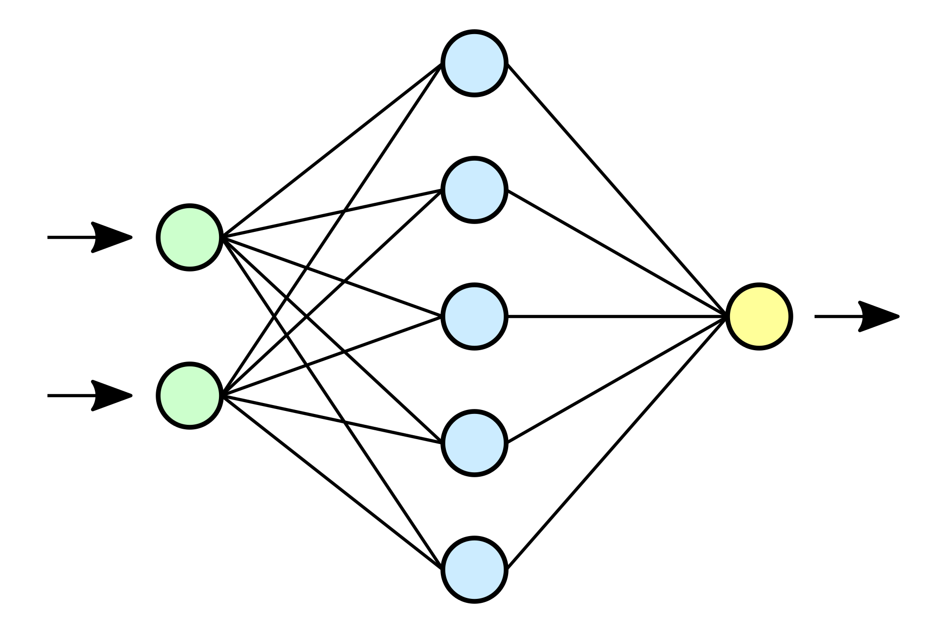
Lets assign some sense to dots and lines.
- Number layers
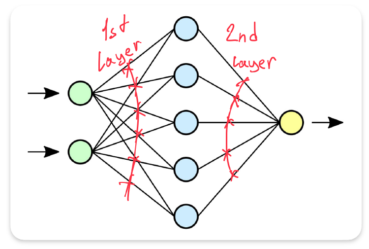
- Single output linear operation
- Matrix form of layer 1
- Matrix form of layer 2
Such pictures always exclude a bias term \(b\). That is why we do not have it in our equations, but we will use it further.
Is that it?
This is 2-layered MLP looks like that?
\[\hat{y} = A(Ax + b) + b\]
It is not. Since linear combination of linear combination is still linear:
\[ \hat{y} = A(Ax + b) + b = AAx + Ab + b, \]
name \(AA = A'\, , \, Ab + b = b'\).
\[ \hat{y} = A(Ax + b) + b = A'x + b'. \]
To obtain final MLP we need a nonlinearity \(\sigma\). Some nonlinear function that is used in between of linear layers to make our neural network capable of learning onlinear relationshions.
Final formula of 2-layered perceptron
\[ \hat{y} = A\big(\sigma(Ax + b)\big) + b. \]
So MLP is a sequence of linear functions with nonlinearity if between of them.
Nonlinearities
Used to be popular: tanh(), sigmoid():
\[\texttt{sigmoid}(x) = \frac{1}{1 + e^{-x}}.\]
Now alternatives of ReLU (rectified linear unit) are used:
\[\texttt{ReLU}(x) = \max(0, x).\]
def relu(x):
    return x * (x > 0)

def sigmoid(x):
    return 1 / (1 + np.exp(x) ** (-1))
x = np.linspace(-10, 10, 100)
_, axes = plt.subplots(1, 2, figsize=(11, 4))
axes[0].plot(x, sigmoid(x))
axes[0].set_title('Sigmoid', fontsize=15)
axes[1].plot(x, relu(x))
axes[1].set_title('ReLU', fontsize=15)
plt.tight_layout()x_torch = torch.linspace(-3, 3, 50)
_, axes = plt.subplots(1, 3, figsize=(15, 4))
axes[0].plot(x_torch, nn.ReLU()(x_torch))
axes[0].plot(x_torch, [0]*50, '--', c='grey')
axes[0].set_title('Torch ReLU', fontsize=15)
axes[1].plot(x_torch, nn.LeakyReLU(0.05)(x_torch))
axes[1].plot(x_torch, [0]*50, '--', c='grey')
axes[1].set_title('Torch Leaky ReLU', fontsize=15)
axes[2].plot(x_torch, nn.GELU()(x_torch))
axes[2].plot(x_torch, [0]*50, '--', c='grey')
axes[2].set_title('Torch GeLU', fontsize=15)
plt.tight_layout()Okay, it looks like that. How does it know things?
Loss functions
Now we have an “arbitrary” function, and we have to solve a minimization problem.
Again, we solve superivsed learning task: \(y\) - observed values, \(\hat{y}\) - approximation with NN.
Our task is find a minimum of a loss function (also called cost or error function). There is a MSE loss:
\[ \mathcal{L}(x) = \frac{1}{N} \sum_1^N \big( y - f(x) \big)^2 \]
And many others for differents tasks. Check them out.
def my_mse(y_true, y_pred):
    dif = y_true - y_pred
    return torch.sum(dif * dif) / len(dif)
y_true = torch.linspace(10, 50, 200)
y_pred = y_true + torch.rand(200) * 25
print(f'My MSE:{my_mse(y_true, y_pred): .5f}')
print(f'Torch MSE:{nn.MSELoss()(y_true, y_pred): .5f}')We want our error to be the smallest possible, so we aim to solve the problem:
\[ \min_x (\mathcal{L}(x)) \]
Gradient descent
Gradient shows the direction of a function growth. Pictures are from wiki.
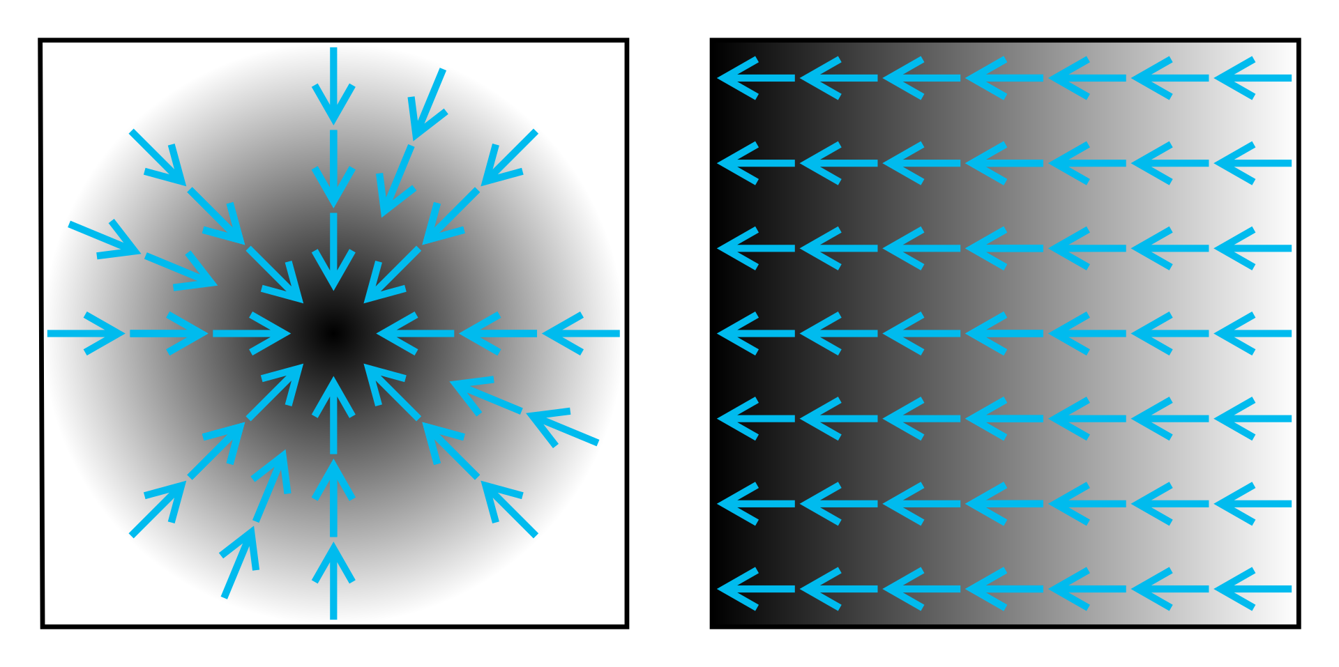
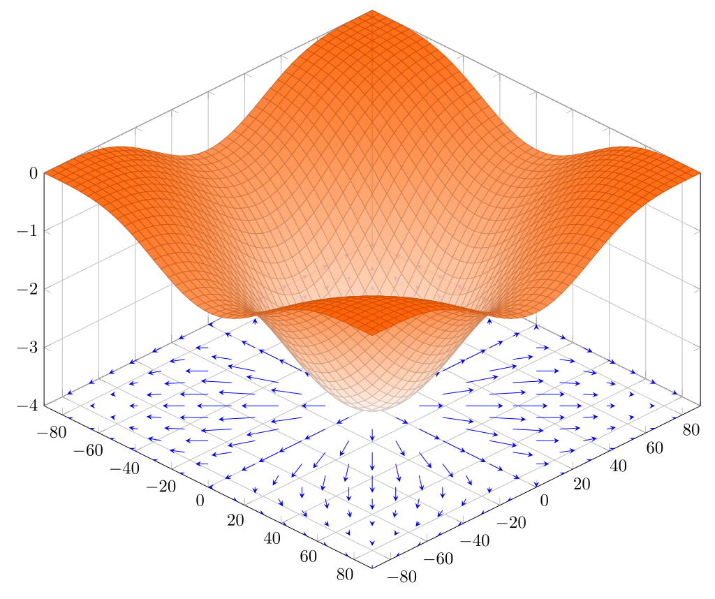
Hence, if we will follow the gradient, we will find the maximum. Let’s go in an opposite direction to the gradient:
\[ x_{i+1} = x_i - \epsilon \nabla f(x), \]
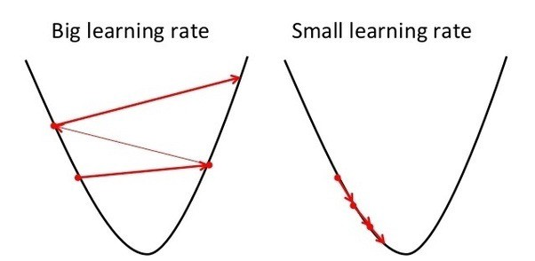
where \(\nabla f(x)\) is a gradient of a function \(f(x)\). \(\epsilon\) is a so-called learning rate. It controls updates: small updates will converge slowly, big updates may mess things up.
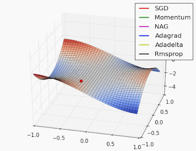
Now there is plenty of gradient descent methods variations. Check this out.
What we actually do with gradient descent is a weight updating
We can say that our NN is parametized by some weights \(\theta\). Then, we would like to get such weights \(\theta\) that will produce the smallest error (i.e. loss):
\[ \theta = \text{argmin}_{\theta} (\mathcal{L}(x, \theta)) \]
And with gradient descent we iteratively update the weights:
\[ \theta_{i+1} = \theta_i - \epsilon \nabla \mathcal{L}(x), \]
With this approach we will obtain such weights that will make our loss (error) function as small as possible, won’t we? Well, theoretically yes…
Universal Approximation Theorem
Based on Cybenko, George. "Approximation by superpositions of a sigmoidal function." Mathematics of control, signals and systems 2.4 (1989): 303-314.
The Universal Approximation Theorem claims that at least one neural network exists that can approximate any continuous function with arbitrary precision. There is quite a few similar theoretical works. Let’s check on Runge’s function:
\[ f(x) = \frac{1}{1 + 25 x^2} \]
def runge_func(x):
    return 1 / (1 + 25 * x * x)
x = torch.linspace(-1, 1, 100)
y = runge_func(x)
plt.plot(x, y, label="Runge's function")
plt.xlabel('x')
plt.ylabel('y')
plt.legend();device = 'cuda:1'# Experiment with this parameters
batch_size = 32 # How many points are treated together by gradient descent?
hidden_neurons = 100 # Number of parameters in the NN
learning_rate = 1e-3 # Step size of gradient descent
n_epochs = 100 # Training duration
num_x_points = 100 # Dataset sizeclass RungesDataset(Dataset):
def __init__(self, n_points):
super(RungesDataset, self).__init__()
self.n_points = n_points
self.x = torch.linspace(-1, 1, n_points)
self.y = runge_func(self.x)
def __len__(self, ):
return self.x.shape[0]
def __getitem__(self, idx):
X, y = self.x[idx], self.y[idx]
return X, y
dataset = RungesDataset(num_x_points)
loader = DataLoader(dataset, batch_size=batch_size, pin_memory=True)# Try different models, losses and optimization methods
model = nn.Sequential(
nn.Linear(1, hidden_neurons, bias=True),
nn.Sigmoid(),
nn.Linear(hidden_neurons, 1, bias=False)
)
opt = torch.optim.Adam(model.parameters(), lr=learning_rate, weight_decay=1e-3)
loss = nn.MSELoss()model = model.to(device)
train_loss = np.array([])
test_loss = np.array([])
for epoch in trange(n_epochs):
loss_epoch_train = np.array([])
loss_epoch_test = np.array([])
model.train(True)
for batch in loader:
X, y = batch[0].unsqueeze(1).to(device), batch[1].unsqueeze(1).to(device)
y_pred = model(X)
l = loss(y_pred, y)
opt.zero_grad()
loss_epoch_train = np.append(loss_epoch_train, l.item())
l.backward()
opt.step()
model.eval()
for batch in loader:
X, y = batch[0].unsqueeze(1).to(device), batch[1].unsqueeze(1).to(device)
y_pred = model(X)
l = loss(y_pred, y)
loss_epoch_test = np.append(loss_epoch_test, l.item())
train_loss = np.append(train_loss, loss_epoch_train.mean())
test_loss = np.append(test_loss, loss_epoch_test.mean())plt.plot(range(n_epochs), train_loss, label='Train')
plt.plot(range(n_epochs), test_loss, label='Test')
plt.legend()
plt.title('Loss');model.eval().cpu()
x_true = torch.linspace(-1, 1, 1000)
plt.plot(x_true, runge_func(x_true), label="Runge's function true")
plt.plot(x_true, model(x_true.reshape(-1, 1)).detach().numpy(), label="Runge's function NN")
plt.xlabel('x')
plt.ylabel('y')
plt.legend();This example does not say that the theorem wrong. Training NN is really sensitive to hyperparameters setup (and such theorems work in specific conditions):
- Not suitable learning. Tuning parameters is such a headache:
- Number of hidden layers
- Dimensionality of hidden layers
- Activation functions
- Weights initialization
- Normalization
- Regularization
- Loss function
- Optimization method
- Parameters of optimization
- Batch size
- Learning procedure
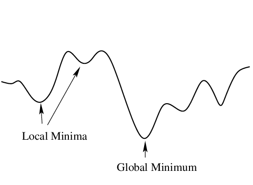
- Problem of finding global minimum in the presence of local minima:
Typically you do not create your own model, but adapt existing one to your problem. In certain cases if you solve a similar problem you may even take the pre-trained model (i.e. you do not train NN by yourself from the very beginning). It is called fine-tuning.
Data vs Task Parallelism
Why GPUs are used?
Data parallelism. You have a large amount of data elements. Each data element (susbet of elements) need to be processed to produce result.
Example: summation of vectors.
Task parallelism. You have collection of tasks that need to be completed.
Example: google chrome and telegram processes.
Automatic Differentiation
Recall gradient descent:
\[ \theta_{i+1} = \theta_i - \epsilon \nabla \mathcal{L}(x). \]
To make a gradient descent we need, well, compute gradients. We may use automatic differentiation packages to compute derivatives. Lets check PyTorch autograd with function:
\[ f(x) = e^{2x}sin(-x)x^2 \, , \]
\[ f'(x) = - xe^{2x}(x\cos(x) + 2\sin(x) + 2x\sin(x)) \, . \]
def some_function(x):
    a = torch.exp(2 * x)
    b = torch.sin(-x)
    c = x * x
    return a * b * c

def deriv_some_function(x):
    a = torch.cos(x) * x
    b = 2 * torch.sin(x)
    c = 2 * torch.sin(x) * x
    tot = - torch.exp(2 * x) * x * (a + b + c)
    return tot
x = torch.tensor(5., requires_grad=True)
y = some_function(x)
print(f'My derivative = {deriv_some_function(x):.3f}')
y.backward()
print(f'Torch derivative = {x.grad:.3f}')x_linspace = torch.linspace(7, 12.3, 1000)
plt.plot(x_linspace, some_function(x_linspace), 'k--', label='Function')
plt.plot(x_linspace, deriv_some_function(x_linspace), label='Analytical deriv')
x_linspace = torch.linspace(7, 12.3, 1000, requires_grad=True)
y_linspace = some_function(x_linspace)
y_sum = torch.sum(y_linspace)
y_sum.backward()
plt.plot(x_linspace.detach().numpy(), x_linspace.grad, label='Torch deriv')
plt.legend();What is going on during one epoch?
An epoch means training the neural network with all the training data for one cycle. In an epoch, we use all of the data exactly once. Learning of a NN may be decomposed on two parts:
- Forward pass. Compute values:
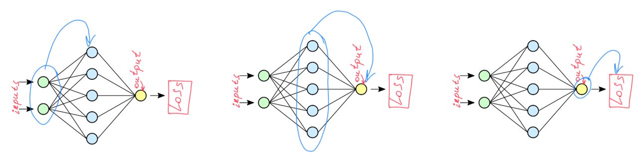
- Backward pass. Compute weights updates:
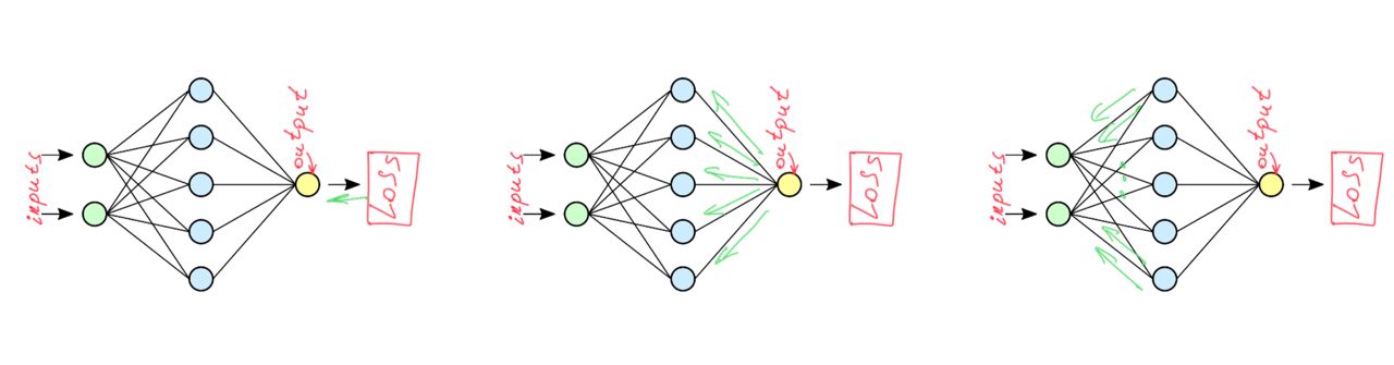
One forward pass and one backward pass are count as one pass.
Recall training in one epoch:
for batch in loader:
    X, y = batch[0].unsqueeze(1).to(device), batch[1].unsqueeze(1).to(device)
    y_pred = model(X)
    l = loss(y_pred, y)

    opt.zero_grad()
    loss_epoch_train = np.append(loss_epoch_train, l.item())
    l.backward()
    opt.step()
In step l.backward(), torch automatically calculates loss derivatives for all weights of our function that requires_grad. In step opt.step(), torch updates the weights with derivatives according to the gradient descent methods used. This is called backpropogation and it is an essence of neural network training.