Danya Merkulov based on the materials from Mikhail Belyaev and Maxim Panov.
🧠 Intuition with k-means
🤔 Problem
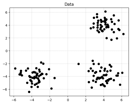
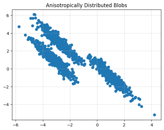
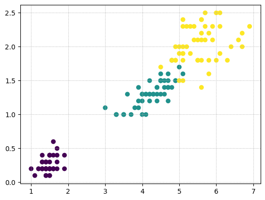
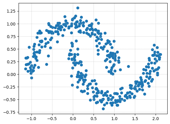
In the scatter plot below, we can see three separate groups of data points and we would like to recover them using clustering.
Think of “discovering” the class labels that we already take for granted in a classification task.
Even if the groups are obvious in the data, it is hard to find them when the data lives in a high-dimensional space, which we can’t visualize in a single histogram or scatterplot.
The \(k\)-means algorithm is a popular clustering method used to partition \(n\) data points into \(k\) clusters. Each data point belongs to the cluster with the closest mean.
Initialization: Randomly select \(k\) data points (or seed them in some other manner) to serve as the initial centroids.
Assignment: Assign each data point to the nearest centroid. The distance is typically computed using the Euclidean distance, though other metrics can be used. Mathematically, assign each data point \(x_i\) to the nearest centroid \(c_j\) using the formula: \[
s(i) = \text{argmin}_{j} \left\| x_i - c_j \right\|^2
\] where \(s(i)\) is the cluster to which data point \(x_i\) is assigned.
Update: Recompute the centroid of each cluster as the mean of all points currently assigned to that cluster. For each cluster \(j\): \[
c_j = \frac{1}{\left| S(j) \right|} \sum_{i \in S(j)} x_i
\] where \(S(j)\) is the set of data points assigned to cluster \(j\).
Convergence: Repeat steps 2 and 3 until the centroids no longer change significantly or some other stopping criteria is met.
Objective Function:
The \(k\)-means algorithm aims to minimize the within-cluster sum of squares (WCSS), given by: \[
J = \sum_{j=1}^{k} \sum_{i \in S(j)} \left\| x_i - c_j \right\|^2
\] Where: - \(J\) is the objective function value (WCSS). - \(k\) is the number of clusters. - \(x_i\) is a data point. - \(c_j\) is the centroid of cluster \(j\).
The goal of the \(k\)-means algorithm is to find the set of centroids \(\{c_1, c_2, ..., c_k\}\) that minimize \(J\).
Notes:
The \(k\)-means algorithm does not guarantee a global optimum solution. The final result might depend on the initial centroids.
To improve the chances of finding a global optimum, the algorithm can be run multiple times with different initializations and the best result (i.e., the one with the lowest WCSS) can be selected.
Question How do you think this could be possibly fixed?
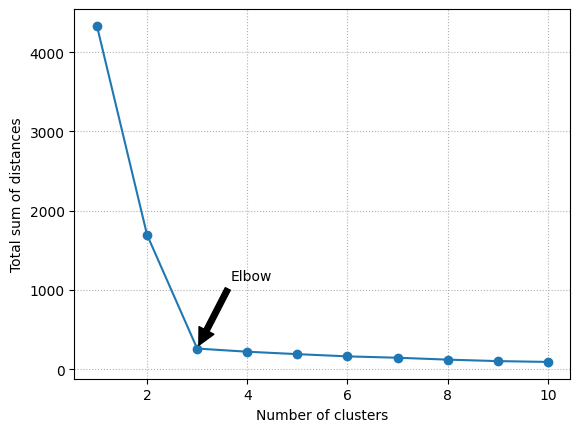
💪 Elbow method
The Elbow method is a “rule-of-thumb” approach to finding the optimal number of clusters.
Here, we look at the cluster variance for different values of k:
import matplotlib.pyplot as pltfrom sklearn.cluster import KMeansdistortions = []for i inrange(1, 11): km = KMeans(n_clusters=i, random_state=1, n_init=10) km.fit(data) distortions.append(km.inertia_)# Plot the distortionsplt.plot(range(1, 11), distortions, "o-")plt.xlabel('Number of clusters')plt.ylabel('Total sum of distances')plt.grid(linestyle=":")# Annotate the point at k=3 with an arrowk =3plt.annotate('Elbow', xy=(k, distortions[k-1]), xytext=(k+1.5, distortions[k-1]+(max(distortions)*0.2)), arrowprops=dict(facecolor='black', shrink=0.05), horizontalalignment='right')plt.show()
Then, we pick the value that resembles the “pit of an elbow.” As we can see, this would be k=3 in this case, which makes sense given our visual expection of the dataset previously.
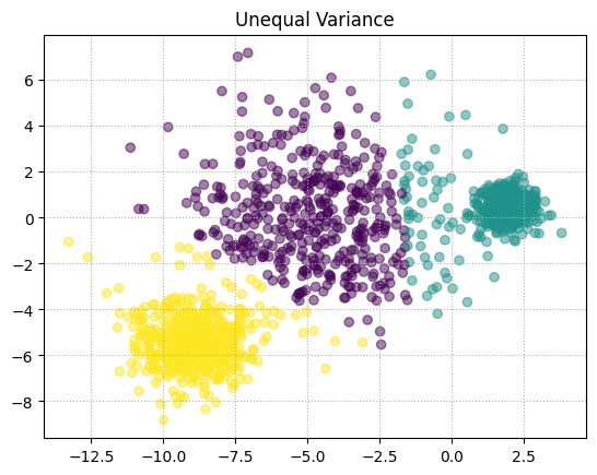
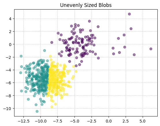
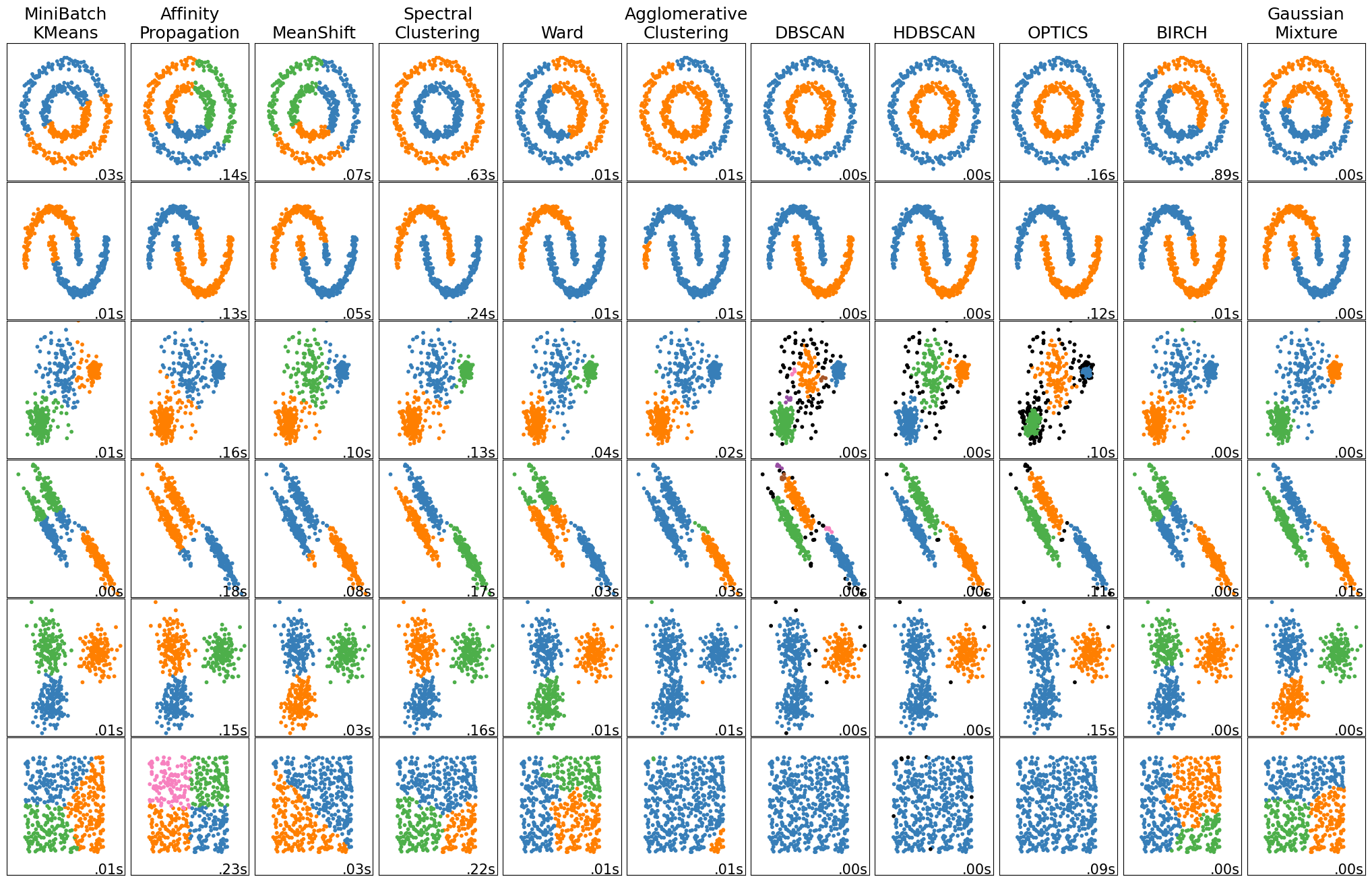
Clustering comes with assumptions: * A clustering algorithm finds clusters by making assumptions with samples should be grouped together. * Each algorithm makes different assumptions and the quality and interpretability of your results will depend on whether the assumptions are satisfied for your goal. * For K-means clustering, the model is that all clusters have equal, spherical variance.
In general, there is no guarantee that structure found by a clustering algorithm has anything to do with what you were interested in.
The following are several well-known clustering algorithms.
sklearn.cluster.KMeans: The simplest, yet effective clustering algorithm. Needs to be provided with the number of clusters in advance, and assumes that the data is normalized as input (but use a PCA model as preprocessor).
sklearn.cluster.MeanShift: Can find better looking clusters than KMeans but is not scalable to high number of samples.
sklearn.cluster.DBSCAN: Can detect irregularly shaped clusters based on density, i.e. sparse regions in the input space are likely to become inter-cluster boundaries. Can also detect outliers (samples that are not part of a cluster).
sklearn.cluster.AffinityPropagation: Clustering algorithm based on message passing between data points.
sklearn.cluster.SpectralClustering: KMeans applied to a projection of the normalized graph Laplacian: finds normalized graph cuts if the affinity matrix is interpreted as an adjacency matrix of a graph.
sklearn.cluster.Ward: Ward implements hierarchical clustering based on the Ward algorithm, a variance-minimizing approach. At each step, it minimizes the sum of squared differences within all clusters (inertia criterion).
Of these, Ward, SpectralClustering, DBSCAN and Affinity propagation can also work with precomputed similarity matrices.
# Source: https://scikit-learn.org/stable/auto_examples/cluster/plot_cluster_comparison.htmlimport timeimport warningsfrom itertools import cycle, isliceimport matplotlib.pyplot as pltimport numpy as npfrom sklearn import cluster, datasets, mixturefrom sklearn.neighbors import kneighbors_graphfrom sklearn.preprocessing import StandardScaler# ============# Generate datasets. We choose the size big enough to see the scalability# of the algorithms, but not too big to avoid too long running times# ============n_samples =500seed =30noisy_circles = datasets.make_circles( n_samples=n_samples, factor=0.5, noise=0.05, random_state=seed)noisy_moons = datasets.make_moons(n_samples=n_samples, noise=0.05, random_state=seed)blobs = datasets.make_blobs(n_samples=n_samples, random_state=seed)rng = np.random.RandomState(seed)no_structure = rng.rand(n_samples, 2), None# Anisotropicly distributed datarandom_state =170X, y = datasets.make_blobs(n_samples=n_samples, random_state=random_state)transformation = [[0.6, -0.6], [-0.4, 0.8]]X_aniso = np.dot(X, transformation)aniso = (X_aniso, y)# blobs with varied variancesvaried = datasets.make_blobs( n_samples=n_samples, cluster_std=[1.0, 2.5, 0.5], random_state=random_state)# ============# Set up cluster parameters# ============plt.figure(figsize=(9*2+3, 13))plt.subplots_adjust( left=0.02, right=0.98, bottom=0.001, top=0.95, wspace=0.05, hspace=0.01)plot_num =1default_base = {"quantile": 0.3,"eps": 0.3,"damping": 0.9,"preference": -200,"n_neighbors": 3,"n_clusters": 3,"min_samples": 7,"xi": 0.05,"min_cluster_size": 0.1,"allow_single_cluster": True,"hdbscan_min_cluster_size": 15,"hdbscan_min_samples": 3,"random_state": 42,}datasets = [ ( noisy_circles, {"damping": 0.77,"preference": -240,"quantile": 0.2,"n_clusters": 2,"min_samples": 7,"xi": 0.08, }, ), ( noisy_moons, {"damping": 0.75,"preference": -220,"n_clusters": 2,"min_samples": 7,"xi": 0.1, }, ), ( varied, {"eps": 0.18,"n_neighbors": 2,"min_samples": 7,"xi": 0.01,"min_cluster_size": 0.2, }, ), ( aniso, {"eps": 0.15,"n_neighbors": 2,"min_samples": 7,"xi": 0.1,"min_cluster_size": 0.2, }, ), (blobs, {"min_samples": 7, "xi": 0.1, "min_cluster_size": 0.2}), (no_structure, {}),]for i_dataset, (dataset, algo_params) inenumerate(datasets):# update parameters with dataset-specific values params = default_base.copy() params.update(algo_params) X, y = dataset# normalize dataset for easier parameter selection X = StandardScaler().fit_transform(X)# estimate bandwidth for mean shift bandwidth = cluster.estimate_bandwidth(X, quantile=params["quantile"])# connectivity matrix for structured Ward connectivity = kneighbors_graph( X, n_neighbors=params["n_neighbors"], include_self=False )# make connectivity symmetric connectivity =0.5* (connectivity + connectivity.T)# ============# Create cluster objects# ============ ms = cluster.MeanShift(bandwidth=bandwidth, bin_seeding=True) two_means = cluster.MiniBatchKMeans( n_clusters=params["n_clusters"], n_init="auto", random_state=params["random_state"], ) ward = cluster.AgglomerativeClustering( n_clusters=params["n_clusters"], linkage="ward", connectivity=connectivity ) spectral = cluster.SpectralClustering( n_clusters=params["n_clusters"], eigen_solver="arpack", affinity="nearest_neighbors", random_state=params["random_state"], ) dbscan = cluster.DBSCAN(eps=params["eps"]) hdbscan = cluster.HDBSCAN( min_samples=params["hdbscan_min_samples"], min_cluster_size=params["hdbscan_min_cluster_size"], allow_single_cluster=params["allow_single_cluster"], ) optics = cluster.OPTICS( min_samples=params["min_samples"], xi=params["xi"], min_cluster_size=params["min_cluster_size"], ) affinity_propagation = cluster.AffinityPropagation( damping=params["damping"], preference=params["preference"], random_state=params["random_state"], ) average_linkage = cluster.AgglomerativeClustering( linkage="average", metric="cityblock", n_clusters=params["n_clusters"], connectivity=connectivity, ) birch = cluster.Birch(n_clusters=params["n_clusters"]) gmm = mixture.GaussianMixture( n_components=params["n_clusters"], covariance_type="full", random_state=params["random_state"], ) clustering_algorithms = ( ("MiniBatch\nKMeans", two_means), ("Affinity\nPropagation", affinity_propagation), ("MeanShift", ms), ("Spectral\nClustering", spectral), ("Ward", ward), ("Agglomerative\nClustering", average_linkage), ("DBSCAN", dbscan), ("HDBSCAN", hdbscan), ("OPTICS", optics), ("BIRCH", birch), ("Gaussian\nMixture", gmm), )for name, algorithm in clustering_algorithms: t0 = time.time()# catch warnings related to kneighbors_graphwith warnings.catch_warnings(): warnings.filterwarnings("ignore", message="the number of connected components of the "+"connectivity matrix is [0-9]{1,2}"+" > 1. Completing it to avoid stopping the tree early.", category=UserWarning, ) warnings.filterwarnings("ignore", message="Graph is not fully connected, spectral embedding"+" may not work as expected.", category=UserWarning, ) algorithm.fit(X) t1 = time.time()ifhasattr(algorithm, "labels_"): y_pred = algorithm.labels_.astype(int)else: y_pred = algorithm.predict(X) plt.subplot(len(datasets), len(clustering_algorithms), plot_num)if i_dataset ==0: plt.title(name, size=18) colors = np.array(list( islice( cycle( ["#377eb8","#ff7f00","#4daf4a","#f781bf","#a65628","#984ea3","#999999","#e41a1c","#dede00", ] ),int(max(y_pred) +1), ) ) )# add black color for outliers (if any) colors = np.append(colors, ["#000000"]) plt.scatter(X[:, 0], X[:, 1], s=10, color=colors[y_pred]) plt.xlim(-2.5, 2.5) plt.ylim(-2.5, 2.5) plt.xticks(()) plt.yticks(()) plt.text(0.99,0.01, ("%.2fs"% (t1 - t0)).lstrip("0"), transform=plt.gca().transAxes, size=15, horizontalalignment="right", ) plot_num +=1plt.show()
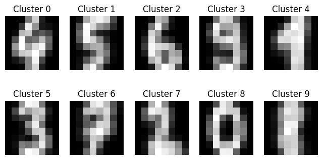
Perform K-means clustering on the digits data, searching for ten clusters.
Visualize the cluster centers as images (i.e. reshape each to 8x8 and use plt.imshow)
Do the clusters seem to be correlated with particular digits?
What is the adjusted_rand_score?
import numpy as npimport matplotlib.pyplot as pltfrom sklearn.cluster import KMeansfrom sklearn.datasets import fetch_openmlfrom sklearn.metrics import adjusted_rand_score# Load the MNIST datasetmnist = fetch_openml('mnist_784', parser="auto")X = mnist.data /255.0# Normalize data to [0, 1]y = mnist.target.astype(int) # Convert target values to integers# Apply K-means clusteringn_clusters =10### 🐱🐱🐱 YOUR CODE HERE 🐱🐱🐱kmeans =None# Visualize the cluster centers as imagesfig, axes = plt.subplots(2, 5, figsize=(8, 4))axes = axes.ravel()for i, center inenumerate(kmeans.cluster_centers_): axes[i].imshow(center.reshape(28, 28), cmap=plt.cm.gray) axes[i].axis('off') axes[i].set_title(f'Cluster {i}')plt.tight_layout()plt.show()3# Do the clusters seem to be correlated with particular digits?# Let's compute the most common label in each clusterlabels = np.zeros_like(kmeans.labels_)for i inrange(n_clusters): mask = (kmeans.labels_ == i) labels[mask] = np.bincount(y[mask]).argmax()# Calculate the adjusted_rand_score### 🐱🐱🐱 YOUR CODE HERE 🐱🐱🐱score =Noneprint(f"Adjusted Rand Score: {score:.4f}")
Try the light version of MNIST (load_digits from sklearn)
from sklearn.datasets import load_digitsdigits = load_digits(n_class=10)digits.data.shape### 🐱🐱🐱 YOUR CODE HERE 🐱🐱🐱kmeans =Noneclusters = kmeans.fit_predict(digits.data)# Visualize the cluster centers as imagesfig, axes = plt.subplots(2, 5, figsize=(8, 4))axes = axes.ravel()for i, center inenumerate(kmeans.cluster_centers_): axes[i].imshow(center.reshape(8, 8), cmap=plt.cm.gray) axes[i].axis('off') axes[i].set_title(f'Cluster {i}')plt.show()### 🐱🐱🐱 YOUR CODE HERE 🐱🐱🐱score =Noneprint(f"Adjusted Rand Score: {score:.4f}")
0.6649258693926379
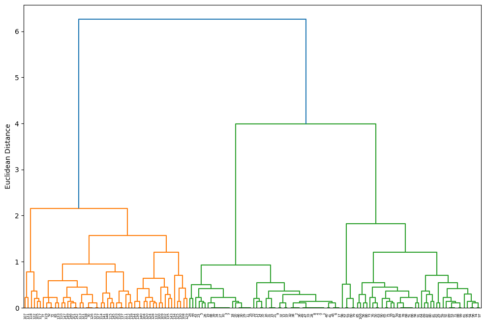
👑 Hierarchical Clustering
One nice feature of hierarchical clustering is that we can visualize the results as a dendrogram, a hierarchical tree.
Using the visualization, we can then decide how “deep” we want to cluster the dataset by setting a “depth” threshold
Or in other words, we don’t need to make a decision about the number of clusters upfront.
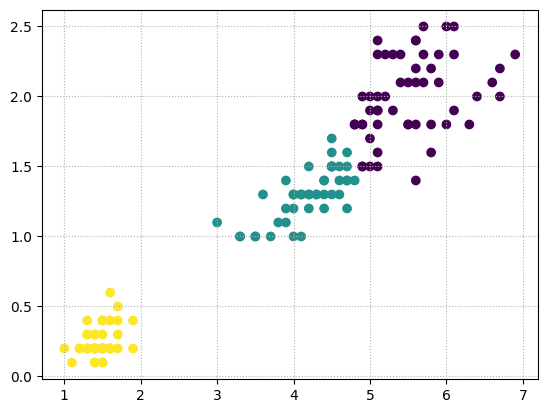
➗ Agglomerative and divisive hierarchical clustering
Furthermore, we can distinguish between 2 main approaches to hierarchical clustering: Divisive clustering and agglomerative clustering.
In agglomerative clustering, we start with a single sample from our dataset and iteratively merge it with other samples to form clusters - we can see it as a bottom-up approach for building the clustering dendrogram.
In divisive clustering, however, we start with the whole dataset as one cluster, and we iteratively split it into smaller subclusters - a top-down approach.
In this notebook, we will use agglomerative clustering.
Single and complete linkage
Now, the next question is how we measure the similarity between samples.
One approach is the familiar Euclidean distance metric that we already used via the K-Means algorithm.
As a refresher, the distance between 2 m-dimensional vectors \(\mathbf{p}\) and \(\mathbf{q}\) can be computed as:
Now, how do we compute the similarity between subclusters of samples?
I.e., our goal is to iteratively merge the most similar pairs of clusters until only one big cluster remains.
There are many different approaches to this, for example single and complete linkage.
In single linkage, we take the pair of the most similar samples (based on the Euclidean distance, for example) in each cluster, and merge the two clusters which have the most similar 2 members into one new, bigger cluster.
In complete linkage, we compare the pairs of the two most dissimilar members of each cluster with each other, and we merge the 2 clusters where the distance between its 2 most dissimilar members is smallest.
/Users/bratishka/.pyenv/versions/3.9.17/envs/benchmarx/lib/python3.9/site-packages/sklearn/cluster/_agglomerative.py:1006: FutureWarning: Attribute `affinity` was deprecated in version 1.2 and will be removed in 1.4. Use `metric` instead
  warnings.warn(
Another useful approach to clustering is Density-based Spatial Clustering of Applications with Noise (DBSCAN).
In essence, we can think of DBSCAN as an algorithm that divides the dataset into subgroup based on dense regions of points.
In DBSCAN, we distinguish between 3 different “points”:
Core points: A core point is a point that has at least a minimum number of other points (MinPts) in its radius epsilon.
Border points: A border point is a point that is not a core point, since it doesn’t have enough MinPts in its neighborhood, but lies within the radius epsilon of a core point.
Noise points: All other points that are neither core points nor border points.
A nice feature about DBSCAN is that we don’t have to specify a number of clusters upfront. However, it requires the setting of additional hyperparameters such as the value for MinPts and the radius epsilon.
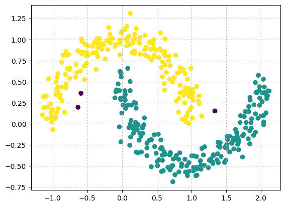
from sklearn.datasets import make_moonsX, y = make_moons(n_samples=400, noise=0.1, random_state=1)plt.scatter(X[:,0], X[:,1])plt.grid(linestyle=":")plt.show()
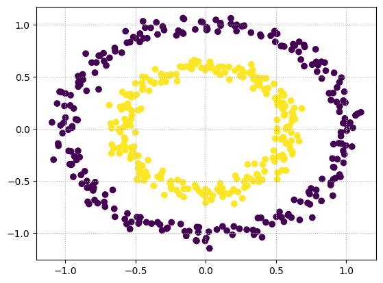
Using the following toy datasets, two concentric circles, experiment with the three different clustering algorithms that we used so far KMeans, AgglomerativeClustering, and DBSCAN.
Which clustering algorithms reproduces or discovers the hidden structure (pretending we don’t know y) best?
Can you explain why this particular algorithm is a good choice while the other 2 “fail”?
from sklearn.datasets import make_circlesX, y = make_circles(n_samples=500, factor=.6, noise=.05)plt.scatter(X[:, 0], X[:, 1], c=y)plt.grid(linestyle=":")plt.show()
### 🐱🐱🐱 YOUR CODE HERE 🐱🐱🐱
💅 Community detection
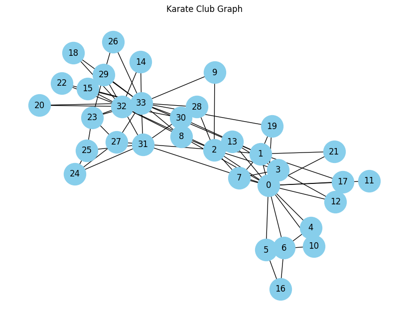
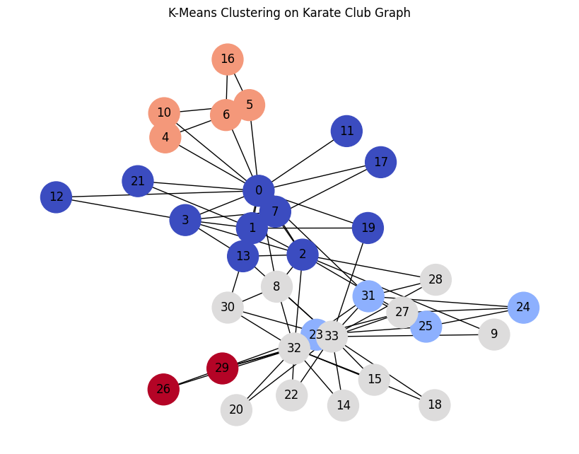
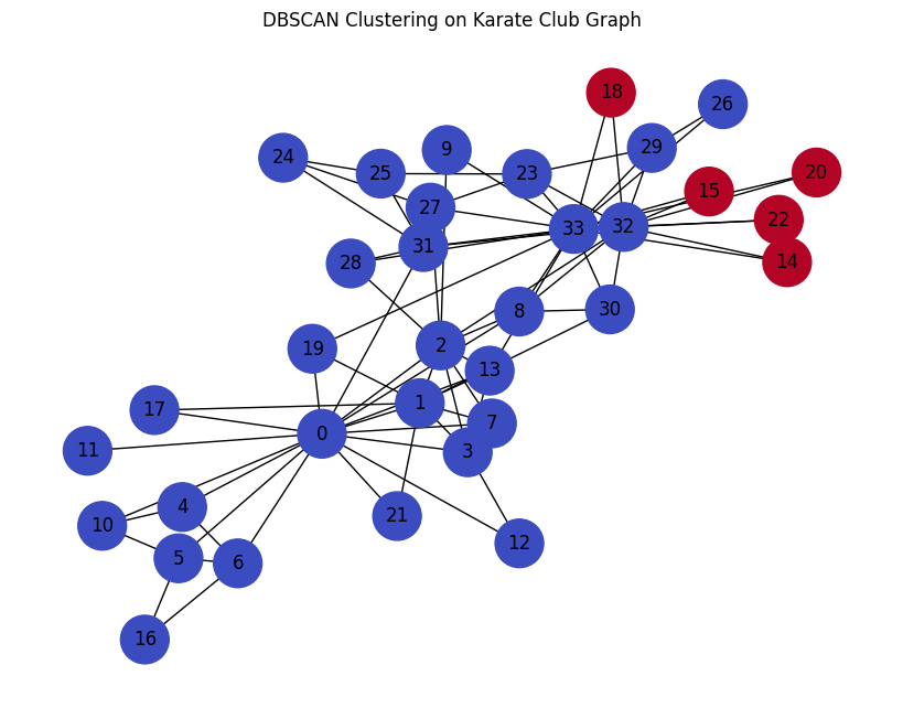
🥋 Karate club
!pip install -q community node2vec python-louvain
import networkx as nximport matplotlib.pyplot as plt# Load the Karate Club graphG = nx.karate_club_graph()# Draw the graphplt.figure(figsize=(8, 6))nx.draw(G, with_labels=True, node_color="skyblue", node_size=1000)plt.title("Karate Club Graph")plt.show()
from node2vec import Node2Vec# Generate embeddings using Node2Vecnode2vec = Node2Vec(G, dimensions=64, walk_length=30, num_walks=200, workers=4)model = node2vec.fit(window=10, min_count=1)# Get embeddings for all nodesembeddings = [model.wv[str(node)] for node in G.nodes()]
from sklearn.cluster import KMeanskmeans = KMeans(n_clusters=5)kmeans_clusters = kmeans.fit_predict(embeddings)# Visualize K-Means clustersplt.figure(figsize=(8, 6))nx.draw(G, with_labels=True, node_color=kmeans_clusters, cmap="coolwarm", node_size=1000)plt.title("K-Means Clustering on Karate Club Graph")plt.show()
/Users/bratishka/.pyenv/versions/3.9.17/envs/benchmarx/lib/python3.9/site-packages/sklearn/cluster/_kmeans.py:1416: FutureWarning: The default value of `n_init` will change from 10 to 'auto' in 1.4. Set the value of `n_init` explicitly to suppress the warning
  super()._check_params_vs_input(X, default_n_init=10)
from sklearn.cluster import DBSCANdbscan = DBSCAN(eps=0.5, min_samples=5)dbscan_clusters = dbscan.fit_predict(embeddings)# Visualize DBSCAN clustersplt.figure(figsize=(8, 6))nx.draw(G, with_labels=True, node_color=dbscan_clusters, cmap="coolwarm", node_size=1000)plt.title("DBSCAN Clustering on Karate Club Graph")plt.show()
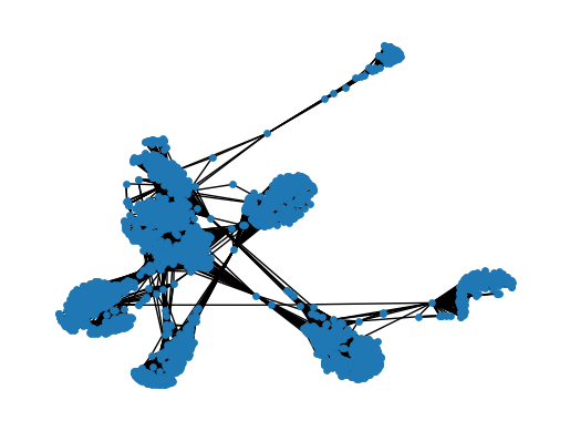
🥺📘 Facebook ego networks
import networkx as nximport requestsimport gzipimport shutilfrom matplotlib import pyplot as plt# Download the dataseturl ="https://snap.stanford.edu/data/facebook_combined.txt.gz"response = requests.get(url, stream=True)withopen("facebook_combined.txt.gz", "wb") asfile:for chunk in response.iter_content(chunk_size=128):file.write(chunk)# Unzip the datasetwith gzip.open("facebook_combined.txt.gz", 'rb') as f_in:withopen("facebook_combined.txt", 'wb') as f_out: shutil.copyfileobj(f_in, f_out)# Load the Facebook graphpath_to_dataset ="facebook_combined.txt"G = nx.read_edgelist(path_to_dataset)print(f"Number of nodes: {G.number_of_nodes()}")print(f"Number of edges: {G.number_of_edges()}")
Number of nodes: 4039
Number of edges: 88234
#Create network layout for visualizationsspring_pos = nx.layout.spring_layout(G)plt.axis("off")nx.draw_networkx(G, pos=spring_pos, with_labels=False, node_size=15)
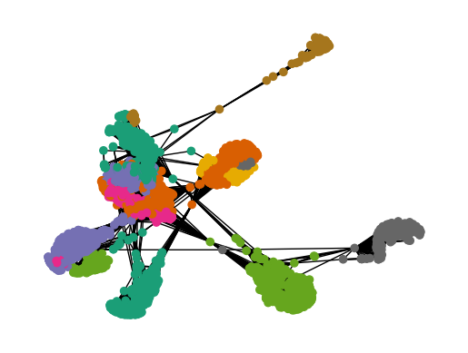
import community as community_louvainparts = community_louvain.best_partition(G)values = [parts.get(node) for node in G.nodes()]
from node2vec import Node2Vec# Generate embeddings using Node2Vecnode2vec = Node2Vec(G, dimensions=128, walk_length=30, num_walks=50, workers=4)model = node2vec.fit(window=10, min_count=1)# Get embeddings for all nodesembeddings = [model.wv[node] for node in G.nodes()]
from sklearn.cluster import KMeanskmeans = KMeans(n_clusters=10) # assuming 10 clusters for demonstrationkmeans_clusters = kmeans.fit_predict(embeddings)
/Users/bratishka/.pyenv/versions/3.9.17/envs/benchmarx/lib/python3.9/site-packages/sklearn/cluster/_kmeans.py:1416: FutureWarning: The default value of `n_init` will change from 10 to 'auto' in 1.4. Set the value of `n_init` explicitly to suppress the warning
  super()._check_params_vs_input(X, default_n_init=10)
from sklearn.cluster import DBSCANdbscan = DBSCAN(eps=0.5, min_samples=5)dbscan_clusters = dbscan.fit_predict(embeddings)
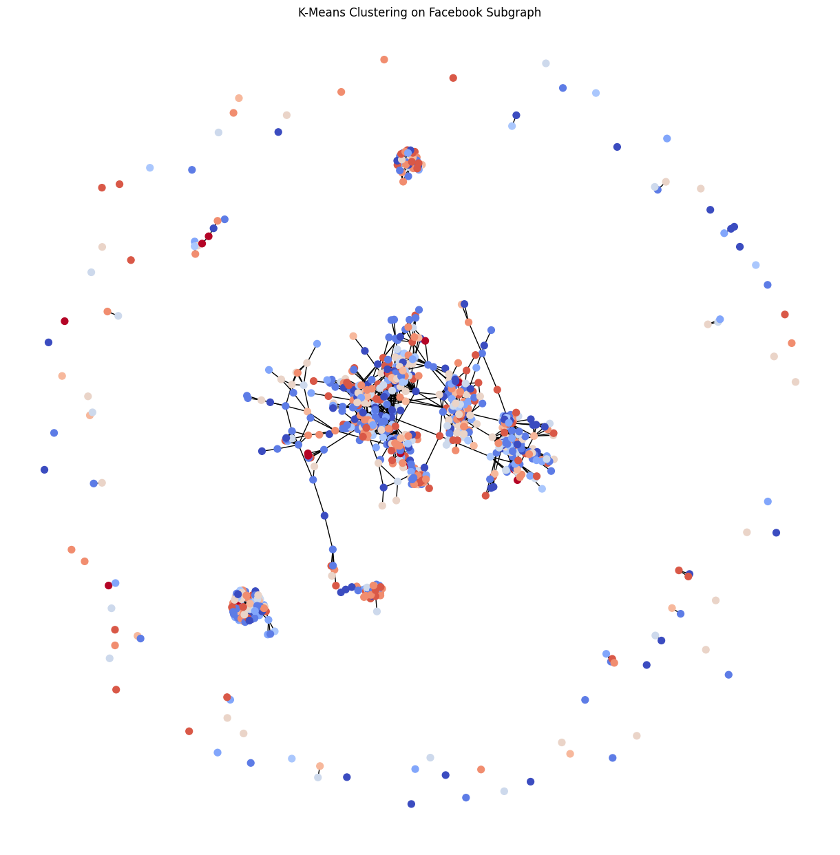
import matplotlib.pyplot as pltimport random# Sample a subgraphsampled_nodes = random.sample(G.nodes(), 1000) # sample 1000 nodessubG = G.subgraph(sampled_nodes)# Get clusters for sampled nodessampled_kmeans_clusters = [kmeans_clusters[int(node)] for node in sampled_nodes]# Visualize K-Means clusters on subgraphplt.figure(figsize=(12, 12))pos = nx.spring_layout(subG)nx.draw(subG, pos, node_color=sampled_kmeans_clusters, cmap="coolwarm", node_size=50)plt.title("K-Means Clustering on Facebook Subgraph")plt.show()
/var/folders/7m/3rbdnx5n5sz625f3l87m91cc0000gn/T/ipykernel_24364/271705878.py:5: DeprecationWarning: Sampling from a set deprecated
since Python 3.9 and will be removed in a subsequent version.
  sampled_nodes = random.sample(G.nodes(), 1000)  # sample 1000 nodes