import matplotlib as mpl
import matplotlib.pyplot as plt
import numpy as np02 Introduction to ML with Python
Matplotlib
A workhorse of scientific visualization in Python.
[deprecated] Set figure appearance in notebook (no pop up).
%matplotlib inlineLine Plot
Draw a line plot of a function
\[ y = x ^2 \]
for \(x\) from -1 to 1.
xs = np.linspace(-1, 1, 101)
ys = xs ** 2
plt.plot(xs, ys, marker='.', color='r', label='$x^2$')
plt.legend()<matplotlib.legend.Legend at 0x7f72b3a4feb0>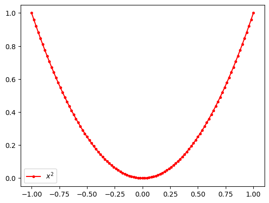
fig, axs = plt.subplots(nrows=1, ncols=2, figsize=(14, 4), layout='constrained')

ax = axs[1]
ax.plot(xs, ys, marker='.', label=r'$x^2$')
ax.plot(xs, np.sqrt(ys), marker='.', label=r'$\sqrt{x^2}$')
ax.legend()
ax.set_xlabel('x')
ax.set_ylabel('y')
ax.grid(True)

plt.show()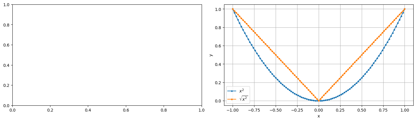
Histogram
cats = np.random.randint(low=0, high=10, size=1000)plt.hist(cats, bins=10, range=(0, 10), width=1.0)
plt.xlabel('Number')
plt.ylabel('Count')Text(0, 0.5, 'Count')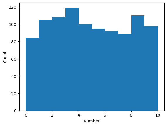
Bar Plot
catsarray([7, 8, 4, 2, 1, 5, 6, 7, 4, 2, 9, 3, 7, 4, 2, 3, 1, 8, 1, 1, 9, 4,
2, 1, 5, 9, 4, 2, 6, 8, 3, 5, 1, 9, 7, 4, 0, 4, 0, 2, 8, 7, 0, 7,
9, 2, 1, 6, 2, 1, 8, 9, 4, 7, 3, 8, 7, 3, 3, 7, 2, 3, 8, 2, 8, 8,
9, 9, 3, 4, 2, 2, 8, 5, 5, 8, 9, 3, 8, 1, 6, 4, 3, 9, 1, 1, 3, 7,
0, 7, 3, 1, 0, 3, 7, 4, 3, 0, 9, 8, 4, 8, 1, 7, 5, 0, 3, 4, 9, 1,
5, 9, 1, 1, 0, 3, 2, 0, 1, 2, 8, 6, 4, 2, 2, 1, 3, 2, 8, 1, 8, 1,
6, 9, 8, 7, 6, 9, 7, 7, 2, 8, 0, 0, 1, 5, 7, 7, 5, 2, 7, 2, 4, 9,
0, 1, 7, 5, 3, 6, 8, 4, 4, 6, 4, 9, 6, 0, 6, 4, 3, 0, 9, 2, 5, 9,
6, 1, 1, 2, 8, 2, 1, 9, 4, 6, 3, 1, 4, 9, 5, 6, 6, 2, 1, 2, 1, 1,
2, 2, 1, 8, 9, 0, 8, 0, 7, 3, 2, 7, 8, 3, 3, 8, 8, 9, 5, 8, 9, 3,
3, 9, 7, 9, 0, 9, 4, 6, 1, 0, 4, 4, 3, 5, 8, 1, 0, 7, 8, 9, 6, 3,
6, 7, 0, 6, 2, 6, 0, 8, 1, 4, 7, 2, 7, 9, 6, 1, 9, 8, 8, 1, 8, 6,
0, 0, 5, 4, 1, 2, 3, 9, 0, 9, 4, 0, 6, 4, 8, 4, 7, 4, 5, 8, 6, 7,
4, 3, 6, 8, 5, 2, 9, 2, 5, 4, 1, 5, 1, 4, 2, 8, 3, 2, 7, 5, 3, 9,
3, 5, 2, 6, 8, 8, 9, 5, 8, 7, 5, 1, 9, 8, 3, 9, 4, 0, 3, 0, 3, 3,
7, 6, 3, 5, 9, 7, 8, 4, 5, 2, 5, 3, 0, 4, 9, 5, 7, 4, 4, 2, 4, 4,
5, 7, 3, 4, 5, 0, 9, 8, 1, 8, 2, 8, 2, 9, 0, 3, 5, 0, 2, 6, 8, 5,
0, 9, 5, 2, 3, 1, 2, 8, 0, 3, 2, 3, 1, 4, 9, 9, 5, 7, 1, 2, 2, 9,
1, 4, 7, 4, 7, 2, 0, 3, 9, 2, 3, 1, 6, 8, 3, 5, 6, 1, 9, 0, 1, 5,
1, 6, 5, 9, 5, 3, 4, 4, 3, 4, 7, 9, 8, 6, 3, 0, 3, 5, 0, 3, 9, 2,
6, 5, 5, 1, 3, 6, 7, 8, 6, 5, 1, 3, 7, 0, 6, 2, 1, 1, 6, 5, 3, 9,
0, 0, 1, 7, 5, 3, 8, 6, 3, 6, 4, 3, 4, 3, 5, 6, 8, 1, 6, 0, 8, 5,
7, 3, 5, 8, 7, 0, 2, 8, 4, 3, 5, 5, 6, 8, 0, 8, 9, 7, 4, 2, 2, 7,
4, 1, 6, 1, 8, 8, 1, 8, 5, 3, 8, 8, 7, 1, 3, 4, 9, 3, 1, 5, 3, 2,
4, 6, 7, 0, 6, 9, 6, 2, 0, 1, 1, 8, 9, 1, 3, 9, 7, 2, 6, 1, 7, 9,
0, 4, 4, 3, 5, 3, 4, 9, 3, 2, 0, 4, 8, 3, 6, 0, 2, 4, 6, 7, 4, 7,
0, 3, 2, 5, 8, 6, 8, 2, 4, 7, 6, 3, 2, 9, 4, 0, 0, 0, 4, 3, 3, 6,
0, 1, 2, 8, 2, 8, 7, 0, 6, 3, 6, 1, 9, 0, 6, 8, 0, 3, 6, 3, 9, 9,
9, 9, 6, 4, 4, 7, 8, 9, 0, 6, 9, 5, 3, 7, 3, 1, 5, 7, 6, 4, 8, 5,
3, 1, 7, 3, 8, 7, 1, 1, 1, 8, 8, 2, 0, 6, 8, 4, 8, 2, 5, 6, 4, 5,
8, 6, 6, 0, 6, 2, 5, 6, 3, 2, 5, 5, 6, 6, 3, 9, 9, 0, 6, 5, 6, 5,
3, 7, 3, 8, 6, 3, 8, 5, 2, 3, 7, 5, 0, 8, 1, 4, 8, 2, 0, 8, 1, 5,
2, 7, 0, 1, 9, 7, 7, 6, 4, 6, 9, 2, 6, 0, 5, 3, 0, 5, 3, 0, 5, 2,
8, 3, 0, 1, 4, 1, 1, 2, 6, 3, 4, 7, 1, 5, 4, 7, 6, 1, 4, 7, 1, 8,
9, 4, 3, 8, 5, 5, 2, 9, 7, 9, 6, 2, 1, 3, 4, 8, 1, 4, 8, 2, 8, 2,
5, 0, 2, 9, 3, 1, 3, 4, 0, 1, 1, 1, 7, 4, 8, 0, 7, 6, 3, 5, 9, 9,
7, 1, 9, 8, 5, 5, 1, 0, 0, 3, 5, 7, 6, 9, 3, 6, 4, 9, 3, 1, 1, 8,
8, 2, 4, 7, 6, 9, 7, 2, 2, 1, 2, 3, 4, 8, 7, 4, 7, 3, 2, 2, 5, 7,
7, 3, 4, 9, 0, 2, 2, 4, 5, 0, 1, 3, 9, 5, 3, 9, 1, 5, 3, 8, 5, 6,
3, 8, 5, 1, 2, 8, 2, 7, 4, 3, 5, 1, 0, 8, 9, 2, 8, 4, 2, 4, 2, 3,
9, 6, 4, 1, 5, 5, 4, 9, 0, 9, 0, 3, 3, 1, 7, 4, 7, 9, 3, 8, 5, 0,
9, 0, 7, 2, 5, 3, 8, 9, 2, 4, 6, 9, 3, 2, 5, 2, 5, 2, 6, 1, 6, 8,
5, 4, 0, 0, 1, 1, 2, 7, 5, 9, 7, 4, 4, 8, 1, 2, 3, 4, 1, 6, 2, 8,
0, 6, 7, 9, 9, 8, 8, 6, 8, 7, 2, 4, 2, 5, 3, 5, 1, 3, 2, 6, 4, 7,
8, 2, 1, 7, 1, 8, 2, 6, 1, 3, 9, 4, 2, 3, 8, 4, 6, 2, 2, 8, 5, 9,
0, 9, 3, 7, 5, 6, 0, 2, 3, 9])counts = np.bincount(cats)
countsarray([ 84, 105, 108, 119, 100, 95, 92, 89, 110, 98])numbers = np.arange(10)plt.bar(numbers, counts)<BarContainer object of 10 artists>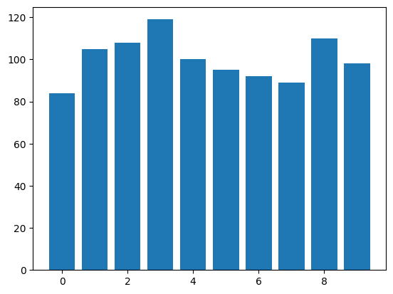
Scatter Plot
Let’s generate random points on a 2D plane and plot them.
n_points = 100
n_dims = 2
xs = np.random.normal(loc=0.0, scale=1.0, size=(n_points, n_dims))
xs.shape(100, 2)xs[:5]array([[ 0.48670473, -0.22935736],
[-1.54387923, -1.16934784],
[-0.47978104, 0.31138709],
[ 0.81350206, -1.09688394],
[-0.54324732, -0.44013888]])plt.scatter(xs[:, 0], xs[:, 1])<matplotlib.collections.PathCollection at 0x7f72b2e7f970>
Sklearn
Toy Problem
Let’s solve a toy problem on a synthetic dataset.
- Generate synthetic dataset.
- Build a model.
- Train a model.
- Evaluate a model.
- Select best model.
Synthetic data
from sklearn.datasets import make_moonsxs, ys = make_moons(n_samples=200, noise=0.1)xs[:5]array([[ 0.67125569, -0.29645975],
[ 1.67693364, -0.31925951],
[ 2.05224091, 0.04264705],
[ 1.77618258, 0.12673704],
[ 1.99973111, 0.3002457 ]])ys[:10]array([1, 1, 1, 1, 1, 1, 0, 0, 1, 0])xs1 = xs[ys == 0]
xs1.shape(100, 2)xs2 = xs[ys == 1]
xs2.shape(100, 2)plt.scatter(xs1[:, 0], xs1[:, 1], label='moon')
plt.scatter(xs2[:, 0], xs2[:, 1], label='dojo cat')
plt.legend()<matplotlib.legend.Legend at 0x7f721002f640>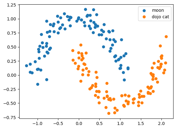
Toy classifier
Train and evaluate a classifier.
from sklearn.linear_model import LogisticRegressionEvery algorithm from sklearn has a set of parameters which could be specified on an instantiation of an estimator.
clf = LogisticRegression(C=10.0)Every algorithm has a method fit.
Signature: estimator.fit(X, y)

Parameters
----------
X : {array-like} of shape (n_samples, n_features)
    Training vectors, where `n_samples` is the number of samples
    and `n_features` is the number of features..

y : array-like of shape (n_samples,)
Target values or classes.xs.shape(200, 2)features = xs
labels = ys
clf.fit(features, labels);A classifier/regressor in sklearn usually has a method .predict() which calculates predictions.
preds = clf.predict(features)predsarray([1, 1, 1, 1, 1, 1, 0, 0, 1, 0, 0, 1, 0, 0, 1, 1, 0, 1, 0, 0, 1, 1,
1, 1, 1, 1, 0, 1, 0, 1, 0, 0, 0, 0, 0, 0, 0, 0, 0, 0, 0, 1, 1, 0,
1, 0, 0, 0, 0, 0, 1, 1, 0, 0, 1, 0, 0, 0, 1, 1, 0, 0, 1, 1, 1, 1,
0, 0, 0, 1, 0, 1, 0, 0, 0, 1, 1, 1, 0, 1, 0, 1, 1, 1, 0, 1, 1, 1,
1, 1, 1, 1, 0, 1, 1, 0, 1, 1, 0, 0, 0, 0, 0, 0, 0, 0, 0, 0, 0, 0,
1, 1, 0, 0, 1, 1, 0, 1, 0, 0, 1, 0, 0, 1, 0, 0, 0, 0, 1, 0, 1, 0,
0, 1, 0, 1, 1, 1, 0, 1, 1, 1, 0, 0, 0, 1, 1, 0, 1, 0, 1, 1, 0, 1,
1, 1, 0, 0, 1, 1, 0, 0, 1, 1, 1, 1, 1, 1, 1, 1, 1, 1, 0, 0, 1, 0,
0, 0, 1, 1, 1, 1, 0, 1, 1, 0, 0, 1, 1, 1, 0, 1, 1, 0, 0, 1, 0, 0,
0, 1])labelsarray([1, 1, 1, 1, 1, 1, 0, 0, 1, 0, 0, 1, 0, 1, 1, 1, 0, 1, 0, 1, 1, 1,
1, 1, 1, 1, 0, 1, 0, 1, 0, 0, 0, 0, 0, 1, 0, 0, 0, 0, 0, 0, 0, 0,
1, 0, 1, 1, 0, 0, 1, 0, 0, 0, 1, 0, 0, 0, 1, 1, 0, 0, 1, 1, 1, 0,
0, 0, 0, 1, 0, 1, 0, 0, 0, 1, 1, 1, 0, 1, 0, 1, 1, 1, 0, 0, 0, 1,
1, 1, 0, 1, 0, 1, 1, 0, 1, 1, 0, 0, 0, 0, 0, 0, 0, 0, 0, 1, 0, 0,
1, 0, 1, 0, 1, 0, 0, 0, 1, 0, 1, 0, 0, 1, 0, 0, 0, 0, 1, 0, 1, 0,
0, 1, 1, 1, 1, 1, 0, 1, 1, 1, 0, 0, 1, 1, 1, 0, 1, 0, 1, 0, 0, 1,
1, 1, 0, 0, 1, 1, 1, 0, 1, 1, 1, 1, 1, 1, 0, 1, 1, 1, 1, 0, 1, 0,
0, 0, 1, 0, 0, 0, 0, 1, 1, 1, 1, 0, 1, 1, 0, 1, 1, 0, 0, 1, 0, 1,
0, 1])def vis(ax: plt.Axes, xs, ys):
xs1 = xs[ys == 0]
xs2 = xs[ys == 1]
ax.scatter(xs1[:, 0], xs1[:, 1], label='moon')
ax.scatter(xs2[:, 0], xs2[:, 1], label='dojo cat')
ax.legend()fig, axs = plt.subplots(nrows=1, ncols=2, figsize=(15, 5))
vis(axs[0], features, labels)
vis(axs[1], features, preds)
plt.show()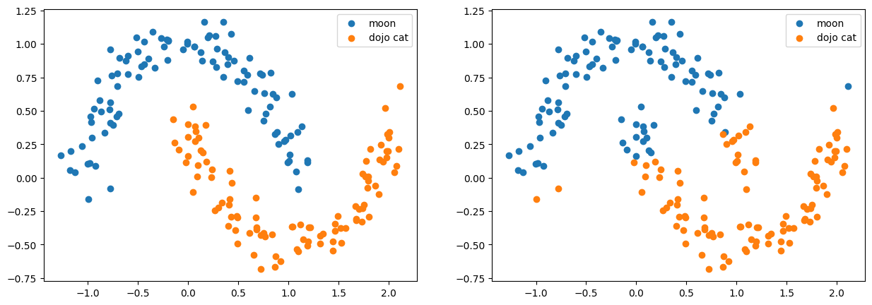
Accuracy
Let’s estimate how accurate our model are. The simplest meature is accuracy metric which is defined as follows.
\[ accuracy = \frac{1}{N} \sum_k^N [y^{(k)}_{true} == y^{(k)}_{pred}] \]
It basically says what percent of target labels we predicted correctly.
from sklearn.metrics import accuracy_scoreaccuracy_score(labels, preds)0.845from sklearn.metrics import classification_reportprint(classification_report(labels, preds)) precision recall f1-score support
0 0.85 0.84 0.84 100
1 0.84 0.85 0.85 100
accuracy 0.84 200
macro avg 0.85 0.84 0.84 200
weighted avg 0.85 0.84 0.84 200
from sklearn.metrics import confusion_matrixconfusion_matrix(labels, preds)array([[84, 16],
[15, 85]])Model Selection
We onl

from sklearn.model_selection import train_test_splitX_train, X_test, y_train, y_test = train_test_split(features, labels, test_size=0.2)X_train.shape(160, 2)X_test.shape(40, 2)clf = LogisticRegression()
clf.fit(X_train, y_train)
y_preds = clf.predict(X_test)y_preds.shape == y_test.shapeTrueaccuracy_score(y_test, y_preds)0.875from sklearn.model_selection import cross_validatecv = cross_validate(clf, features, labels, cv=3, scoring=['accuracy', 'precision', 'recall'])
cv{'fit_time': array([0.00665188, 0.00604677, 0.00470114]),
'score_time': array([0.01224828, 0.01190948, 0.00847197]),
'test_accuracy': array([0.88059701, 0.82089552, 0.84848485]),
'test_precision': array([0.93333333, 0.8 , 0.82857143]),
'test_recall': array([0.82352941, 0.84848485, 0.87878788])}cv['test_accuracy'].mean()0.8499924619327605Bridging to pandas
Dictionary is not very convinient for post processing of data. Let’s convert it to pandas.DataFraem and make couple of tricks.
import pandas as pddf = pd.DataFrame(cv)
df| fit_time | score_time | test_accuracy | test_precision | test_recall | |
|---|---|---|---|---|---|
| 0 | 0.006652 | 0.012248 | 0.880597 | 0.933333 | 0.823529 |
| 1 | 0.006047 | 0.011909 | 0.820896 | 0.800000 | 0.848485 |
| 2 | 0.004701 | 0.008472 | 0.848485 | 0.828571 | 0.878788 |
df = df[df.columns[2:]]
df| test_accuracy | test_precision | test_recall | |
|---|---|---|---|
| 0 | 0.880597 | 0.933333 | 0.823529 |
| 1 | 0.820896 | 0.800000 | 0.848485 |
| 2 | 0.848485 | 0.828571 | 0.878788 |
df.mean()test_accuracy 0.849992
test_precision 0.853968
test_recall 0.850267
dtype: float64Pandas
The most usefull and commonly used library for tabular data.
import numpy as np
import pandas as pd
url = 'https://raw.github.com/mattdelhey/kaggle-titanic/master/Data/train.csv'titanic = pd.read_csv(url)
titanic.info()<class 'pandas.core.frame.DataFrame'>
RangeIndex: 891 entries, 0 to 890
Data columns (total 11 columns):
# Column Non-Null Count Dtype
--- ------ -------------- -----
0 survived 891 non-null int64
1 pclass 891 non-null int64
2 name 891 non-null object
3 sex 891 non-null object
4 age 714 non-null float64
5 sibsp 891 non-null int64
6 parch 891 non-null int64
7 ticket 891 non-null object
8 fare 891 non-null float64
9 cabin 204 non-null object
10 embarked 889 non-null object
dtypes: float64(2), int64(4), object(5)
memory usage: 76.7+ KBtitanic| survived | pclass | name | sex | age | sibsp | parch | ticket | fare | cabin | embarked | |
|---|---|---|---|---|---|---|---|---|---|---|---|
| 0 | 0 | 3 | Braund, Mr. Owen Harris | male | 22.0 | 1 | 0 | A/5 21171 | 7.2500 | NaN | S |
| 1 | 1 | 1 | Cumings, Mrs. John Bradley (Florence Briggs Th... | female | 38.0 | 1 | 0 | PC 17599 | 71.2833 | C85 | C |
| 2 | 1 | 3 | Heikkinen, Miss. Laina | female | 26.0 | 0 | 0 | STON/O2. 3101282 | 7.9250 | NaN | S |
| 3 | 1 | 1 | Futrelle, Mrs. Jacques Heath (Lily May Peel) | female | 35.0 | 1 | 0 | 113803 | 53.1000 | C123 | S |
| 4 | 0 | 3 | Allen, Mr. William Henry | male | 35.0 | 0 | 0 | 373450 | 8.0500 | NaN | S |
| ... | ... | ... | ... | ... | ... | ... | ... | ... | ... | ... | ... |
| 886 | 0 | 2 | Montvila, Rev. Juozas | male | 27.0 | 0 | 0 | 211536 | 13.0000 | NaN | S |
| 887 | 1 | 1 | Graham, Miss. Margaret Edith | female | 19.0 | 0 | 0 | 112053 | 30.0000 | B42 | S |
| 888 | 0 | 3 | Johnston, Miss. Catherine Helen "Carrie" | female | NaN | 1 | 2 | W./C. 6607 | 23.4500 | NaN | S |
| 889 | 1 | 1 | Behr, Mr. Karl Howell | male | 26.0 | 0 | 0 | 111369 | 30.0000 | C148 | C |
| 890 | 0 | 3 | Dooley, Mr. Patrick | male | 32.0 | 0 | 0 | 370376 | 7.7500 | NaN | Q |
891 rows × 11 columns
titanic.describe()| survived | pclass | age | sibsp | parch | fare | |
|---|---|---|---|---|---|---|
| count | 891.000000 | 891.000000 | 714.000000 | 891.000000 | 891.000000 | 891.000000 |
| mean | 0.383838 | 2.308642 | 29.699118 | 0.523008 | 0.381594 | 32.204208 |
| std | 0.486592 | 0.836071 | 14.526497 | 1.102743 | 0.806057 | 49.693429 |
| min | 0.000000 | 1.000000 | 0.420000 | 0.000000 | 0.000000 | 0.000000 |
| 25% | 0.000000 | 2.000000 | 20.125000 | 0.000000 | 0.000000 | 7.910400 |
| 50% | 0.000000 | 3.000000 | 28.000000 | 0.000000 | 0.000000 | 14.454200 |
| 75% | 1.000000 | 3.000000 | 38.000000 | 1.000000 | 0.000000 | 31.000000 |
| max | 1.000000 | 3.000000 | 80.000000 | 8.000000 | 6.000000 | 512.329200 |
titanic.sort_values(by='age', ascending=False).head(5)| survived | pclass | name | sex | age | sibsp | parch | ticket | fare | cabin | embarked | |
|---|---|---|---|---|---|---|---|---|---|---|---|
| 630 | 1 | 1 | Barkworth, Mr. Algernon Henry Wilson | male | 80.0 | 0 | 0 | 27042 | 30.0000 | A23 | S |
| 851 | 0 | 3 | Svensson, Mr. Johan | male | 74.0 | 0 | 0 | 347060 | 7.7750 | NaN | S |
| 493 | 0 | 1 | Artagaveytia, Mr. Ramon | male | 71.0 | 0 | 0 | PC 17609 | 49.5042 | NaN | C |
| 96 | 0 | 1 | Goldschmidt, Mr. George B | male | 71.0 | 0 | 0 | PC 17754 | 34.6542 | A5 | C |
| 116 | 0 | 3 | Connors, Mr. Patrick | male | 70.5 | 0 | 0 | 370369 | 7.7500 | NaN | Q |
Indexing can be tricky.
titanic[['age', 'name']].head(5)| age | name | |
|---|---|---|
| 0 | 22.0 | Braund, Mr. Owen Harris |
| 1 | 38.0 | Cumings, Mrs. John Bradley (Florence Briggs Th... |
| 2 | 26.0 | Heikkinen, Miss. Laina |
| 3 | 35.0 | Futrelle, Mrs. Jacques Heath (Lily May Peel) |
| 4 | 35.0 | Allen, Mr. William Henry |
titanic.iloc[:5]| survived | pclass | name | sex | age | sibsp | parch | ticket | fare | cabin | embarked | |
|---|---|---|---|---|---|---|---|---|---|---|---|
| 0 | 0 | 3 | Braund, Mr. Owen Harris | male | 22.0 | 1 | 0 | A/5 21171 | 7.2500 | NaN | S |
| 1 | 1 | 1 | Cumings, Mrs. John Bradley (Florence Briggs Th... | female | 38.0 | 1 | 0 | PC 17599 | 71.2833 | C85 | C |
| 2 | 1 | 3 | Heikkinen, Miss. Laina | female | 26.0 | 0 | 0 | STON/O2. 3101282 | 7.9250 | NaN | S |
| 3 | 1 | 1 | Futrelle, Mrs. Jacques Heath (Lily May Peel) | female | 35.0 | 1 | 0 | 113803 | 53.1000 | C123 | S |
| 4 | 0 | 3 | Allen, Mr. William Henry | male | 35.0 | 0 | 0 | 373450 | 8.0500 | NaN | S |
titanic.iloc[[2, 5, 6], 2:5]| name | sex | age | |
|---|---|---|---|
| 2 | Heikkinen, Miss. Laina | female | 26.0 |
| 5 | Moran, Mr. James | male | NaN |
| 6 | McCarthy, Mr. Timothy J | male | 54.0 |
df = titanic.set_index('ticket')df = df.sort_index()df.loc['W./C. 6609']survived 0
pclass 3
name Harknett, Miss. Alice Phoebe
sex female
age NaN
sibsp 0
parch 0
fare 7.55
cabin NaN
embarked S
Name: W./C. 6609, dtype: objectdf| survived | pclass | name | sex | age | sibsp | parch | fare | cabin | embarked | |
|---|---|---|---|---|---|---|---|---|---|---|
| ticket | ||||||||||
| 110152 | 1 | 1 | Maioni, Miss. Roberta | female | 16.0 | 0 | 0 | 86.500 | B79 | S |
| 110152 | 1 | 1 | Cherry, Miss. Gladys | female | 30.0 | 0 | 0 | 86.500 | B77 | S |
| 110152 | 1 | 1 | Rothes, the Countess. of (Lucy Noel Martha Dye... | female | 33.0 | 0 | 0 | 86.500 | B77 | S |
| 110413 | 0 | 1 | Taussig, Mr. Emil | male | 52.0 | 1 | 1 | 79.650 | E67 | S |
| 110413 | 1 | 1 | Taussig, Mrs. Emil (Tillie Mandelbaum) | female | 39.0 | 1 | 1 | 79.650 | E67 | S |
| ... | ... | ... | ... | ... | ... | ... | ... | ... | ... | ... |
| W./C. 6609 | 0 | 3 | Harknett, Miss. Alice Phoebe | female | NaN | 0 | 0 | 7.550 | NaN | S |
| W.E.P. 5734 | 0 | 1 | Chaffee, Mr. Herbert Fuller | male | 46.0 | 1 | 0 | 61.175 | E31 | S |
| W/C 14208 | 0 | 2 | Harris, Mr. Walter | male | 30.0 | 0 | 0 | 10.500 | NaN | S |
| WE/P 5735 | 1 | 1 | Crosby, Miss. Harriet R | female | 36.0 | 0 | 2 | 71.000 | B22 | S |
| WE/P 5735 | 0 | 1 | Crosby, Capt. Edward Gifford | male | 70.0 | 1 | 1 | 71.000 | B22 | S |
891 rows × 10 columns
type(titanic)pandas.core.frame.DataFrametype(titanic.age)pandas.core.series.Seriestitanic['age']0 22.0
1 38.0
2 26.0
3 35.0
4 35.0
...
886 27.0
887 19.0
888 NaN
889 26.0
890 32.0
Name: age, Length: 891, dtype: float64You can extract a numpy array
type(titanic.values)  # depracted
type(titanic.to_numpy())titanic.age.to_numpy()[:10]titanic.age.to_numpy()See more details here: 10 Minutes to pandas (actually it requires much more)
http://pandas.pydata.org/pandas-docs/stable/10min.html
Seaborn
A high-level library for visualization and exploratory data analysis.
!pip install seabornRequirement already satisfied: seaborn in /usr/local/lib/python3.10/dist-packages (0.13.0)
Requirement already satisfied: matplotlib!=3.6.1,>=3.3 in /usr/local/lib/python3.10/dist-packages (from seaborn) (3.8.0)
Requirement already satisfied: numpy!=1.24.0,>=1.20 in /usr/local/lib/python3.10/dist-packages (from seaborn) (1.26.0)
Requirement already satisfied: pandas>=1.2 in /usr/local/lib/python3.10/dist-packages (from seaborn) (2.1.1)
Requirement already satisfied: pyparsing>=2.3.1 in /usr/local/lib/python3.10/dist-packages (from matplotlib!=3.6.1,>=3.3->seaborn) (3.1.1)
Requirement already satisfied: fonttools>=4.22.0 in /usr/local/lib/python3.10/dist-packages (from matplotlib!=3.6.1,>=3.3->seaborn) (4.43.0)
Requirement already satisfied: kiwisolver>=1.0.1 in /usr/local/lib/python3.10/dist-packages (from matplotlib!=3.6.1,>=3.3->seaborn) (1.4.5)
Requirement already satisfied: python-dateutil>=2.7 in /usr/local/lib/python3.10/dist-packages (from matplotlib!=3.6.1,>=3.3->seaborn) (2.8.2)
Requirement already satisfied: pillow>=6.2.0 in /usr/local/lib/python3.10/dist-packages (from matplotlib!=3.6.1,>=3.3->seaborn) (10.0.1)
Requirement already satisfied: packaging>=20.0 in /usr/local/lib/python3.10/dist-packages (from matplotlib!=3.6.1,>=3.3->seaborn) (23.2)
Requirement already satisfied: cycler>=0.10 in /usr/local/lib/python3.10/dist-packages (from matplotlib!=3.6.1,>=3.3->seaborn) (0.12.0)
Requirement already satisfied: contourpy>=1.0.1 in /usr/local/lib/python3.10/dist-packages (from matplotlib!=3.6.1,>=3.3->seaborn) (1.1.1)
Requirement already satisfied: pytz>=2020.1 in /usr/local/lib/python3.10/dist-packages (from pandas>=1.2->seaborn) (2023.3.post1)
Requirement already satisfied: tzdata>=2022.1 in /usr/local/lib/python3.10/dist-packages (from pandas>=1.2->seaborn) (2023.3)
Requirement already satisfied: six>=1.5 in /usr/local/lib/python3.10/dist-packages (from python-dateutil>=2.7->matplotlib!=3.6.1,>=3.3->seaborn) (1.16.0)
WARNING: Running pip as the 'root' user can result in broken permissions and conflicting behaviour with the system package manager. It is recommended to use a virtual environment instead: https://pip.pypa.io/warnings/venvimport seaborn as sns# sns.set() allows to use a more attractive color scheme for plots
sns.set()sns.catplot(x="pclass", kind="count", data=titanic)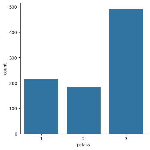
sns.catplot(titanic, x="pclass", hue="sex", kind="count")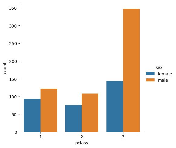
fg = sns.FacetGrid(titanic, hue="sex", aspect=3)
fg.map(sns.kdeplot, "age", fill=True)
fg.set(xlim=(0, 80));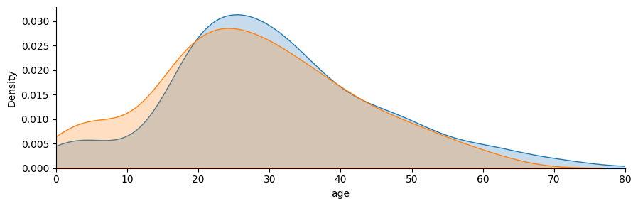
fg = sns.FacetGrid(titanic, col="sex", row="pclass", hue="sex", height=2.5, aspect=2.5)
fg.map(sns.kdeplot, "age", fill=True)
fg.map(sns.rugplot, "age")
sns.despine(left=True)
fg.set(xlim=(0, 80));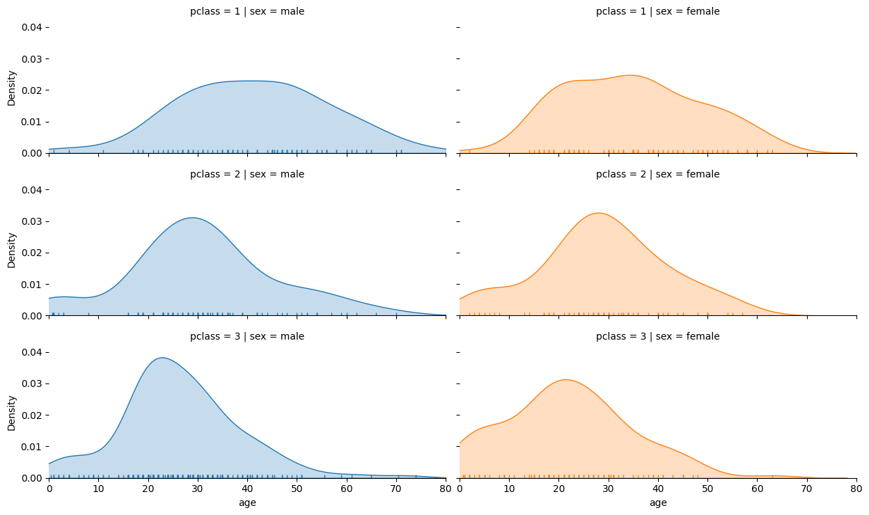
Visualising the survival of passengers based on classes.
grid = sns.FacetGrid(titanic, col='survived', row='pclass', height=2.2, aspect=1.6)
grid.map(plt.hist, 'age', alpha=.5, bins=20)
grid.add_legend();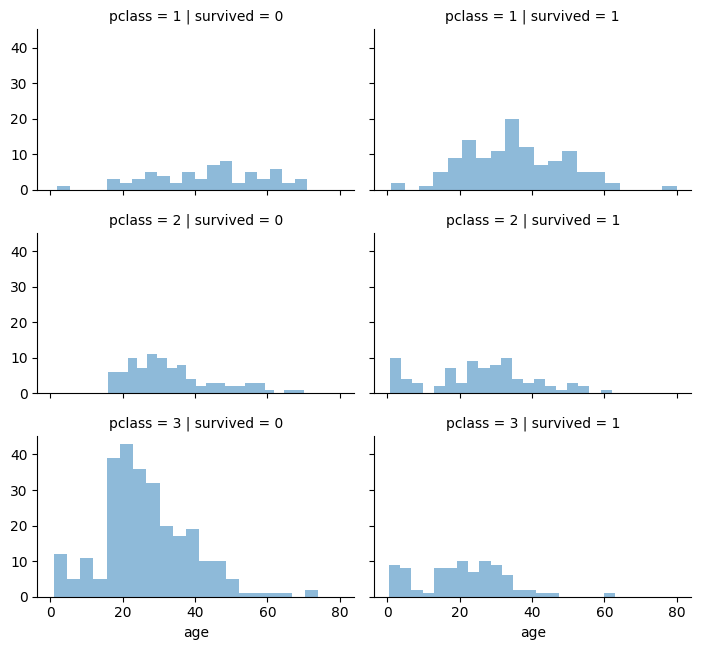
Visualising Class and Embarkment with Survivability.
grid = sns.FacetGrid(titanic, row ='embarked', height=4, aspect=3)
grid.map(sns.pointplot, 'pclass', 'survived', 'sex', palette='deep')
grid.add_legend()
/usr/local/lib/python3.10/dist-packages/seaborn/axisgrid.py:718: UserWarning: Using the pointplot function without specifying `order` is likely to produce an incorrect plot.
warnings.warn(warning)
/usr/local/lib/python3.10/dist-packages/seaborn/axisgrid.py:723: UserWarning: Using the pointplot function without specifying `hue_order` is likely to produce an incorrect plot.
warnings.warn(warning)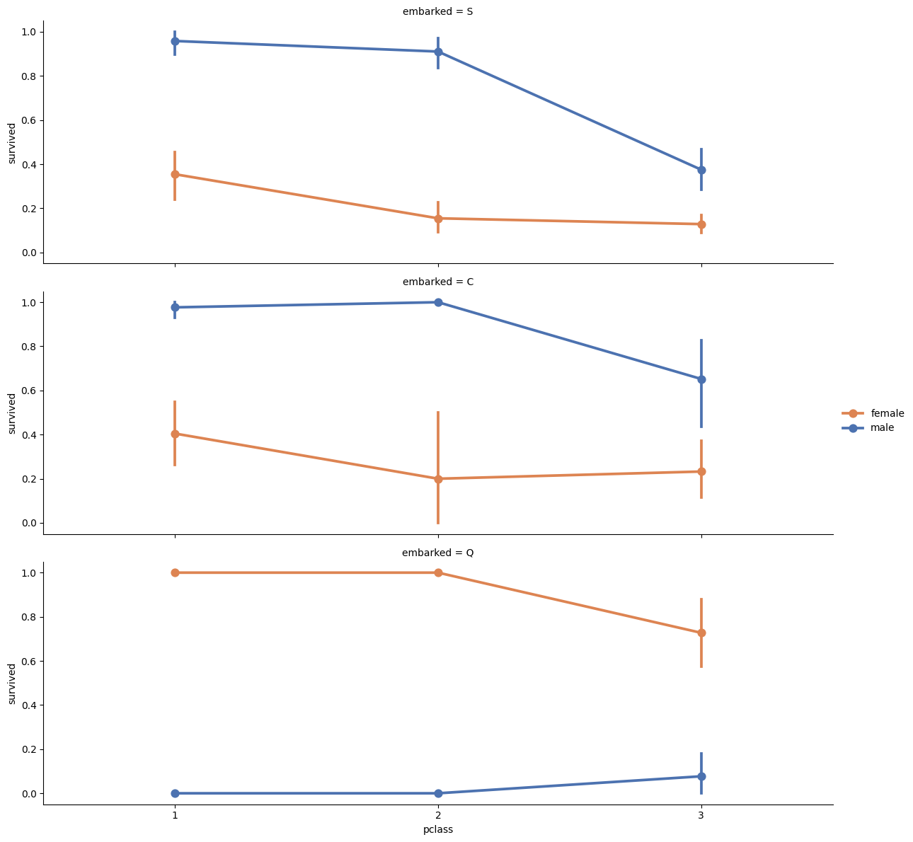
See more example of Seaborn visualizations for the Titanic dataset here
https://gist.github.com/mwaskom/8224591
Model Problem
- Load data from the csv file.
- Check column names.
- Look for dependencies between features and the target vector.
Public Kaggle competition is here (for those who want compete for fun).
Data Preprocessing
from sklearn.neighbors import KNeighborsClassifierLet’s do little bit of processing to make some different variables that might be more interesting to plot. Since this notebook is focused on visualization, we’re going to do this without much comment.
titanic = titanic.drop(['name', 'ticket', 'cabin'], axis=1)
titanic['sex'] = titanic.sex.map({'male': 0, 'female': 1})
titanic = pd.get_dummies(titanic, dummy_na=True, columns=['embarked'])
titanic.head()| survived | pclass | sex | age | sibsp | parch | fare | embarked_C | embarked_Q | embarked_S | embarked_nan | |
|---|---|---|---|---|---|---|---|---|---|---|---|
| 0 | 0 | 3 | 0 | 22.0 | 1 | 0 | 7.2500 | False | False | True | False |
| 1 | 1 | 1 | 1 | 38.0 | 1 | 0 | 71.2833 | True | False | False | False |
| 2 | 1 | 3 | 1 | 26.0 | 0 | 0 | 7.9250 | False | False | True | False |
| 3 | 1 | 1 | 1 | 35.0 | 1 | 0 | 53.1000 | False | False | True | False |
| 4 | 0 | 3 | 0 | 35.0 | 0 | 0 | 8.0500 | False | False | True | False |
titanic[titanic.columns[:7]]| survived | pclass | sex | age | sibsp | parch | fare | |
|---|---|---|---|---|---|---|---|
| 0 | 0 | 3 | 0 | 22.0 | 1 | 0 | 7.2500 |
| 1 | 1 | 1 | 1 | 38.0 | 1 | 0 | 71.2833 |
| 2 | 1 | 3 | 1 | 26.0 | 0 | 0 | 7.9250 |
| 3 | 1 | 1 | 1 | 35.0 | 1 | 0 | 53.1000 |
| 4 | 0 | 3 | 0 | 35.0 | 0 | 0 | 8.0500 |
| ... | ... | ... | ... | ... | ... | ... | ... |
| 885 | 0 | 3 | 1 | 39.0 | 0 | 5 | 29.1250 |
| 886 | 0 | 2 | 0 | 27.0 | 0 | 0 | 13.0000 |
| 887 | 1 | 1 | 1 | 19.0 | 0 | 0 | 30.0000 |
| 889 | 1 | 1 | 0 | 26.0 | 0 | 0 | 30.0000 |
| 890 | 0 | 3 | 0 | 32.0 | 0 | 0 | 7.7500 |
714 rows × 7 columns
titanic.count()survived 891
pclass 891
sex 891
age 714
sibsp 891
parch 891
fare 891
embarked_C 891
embarked_Q 891
embarked_S 891
embarked_nan 891
dtype: int64# titanic.dropna(inplace=True)
titanic = titanic.dropna()
titanic.head(6)| survived | pclass | sex | age | sibsp | parch | fare | embarked_C | embarked_Q | embarked_S | embarked_nan | |
|---|---|---|---|---|---|---|---|---|---|---|---|
| 0 | 0 | 3 | 0 | 22.0 | 1 | 0 | 7.2500 | False | False | True | False |
| 1 | 1 | 1 | 1 | 38.0 | 1 | 0 | 71.2833 | True | False | False | False |
| 2 | 1 | 3 | 1 | 26.0 | 0 | 0 | 7.9250 | False | False | True | False |
| 3 | 1 | 1 | 1 | 35.0 | 1 | 0 | 53.1000 | False | False | True | False |
| 4 | 0 | 3 | 0 | 35.0 | 0 | 0 | 8.0500 | False | False | True | False |
| 6 | 0 | 1 | 0 | 54.0 | 0 | 0 | 51.8625 | False | False | True | False |
titanic.count()survived 714
pclass 714
sex 714
age 714
sibsp 714
parch 714
fare 714
embarked_C 714
embarked_Q 714
embarked_S 714
embarked_nan 714
dtype: int64Our target value is wheter passnager survice or not (survived). The rest of columns are features.
titanic = titanic[titanic.columns[:7]]
titanic| survived | pclass | sex | age | sibsp | parch | fare | |
|---|---|---|---|---|---|---|---|
| 0 | 0 | 3 | 0 | 22.0 | 1 | 0 | 7.2500 |
| 1 | 1 | 1 | 1 | 38.0 | 1 | 0 | 71.2833 |
| 2 | 1 | 3 | 1 | 26.0 | 0 | 0 | 7.9250 |
| 3 | 1 | 1 | 1 | 35.0 | 1 | 0 | 53.1000 |
| 4 | 0 | 3 | 0 | 35.0 | 0 | 0 | 8.0500 |
| ... | ... | ... | ... | ... | ... | ... | ... |
| 885 | 0 | 3 | 1 | 39.0 | 0 | 5 | 29.1250 |
| 886 | 0 | 2 | 0 | 27.0 | 0 | 0 | 13.0000 |
| 887 | 1 | 1 | 1 | 19.0 | 0 | 0 | 30.0000 |
| 889 | 1 | 1 | 0 | 26.0 | 0 | 0 | 30.0000 |
| 890 | 0 | 3 | 0 | 32.0 | 0 | 0 | 7.7500 |
714 rows × 7 columns
# extract X - features & y - targets
X = titanic.drop('survived', axis=1)
y = titanic.survived
Now it’s time to build a model
# initialize a classifier
clf = KNeighborsClassifier()

# train the classifier
clf.fit(X, y)

# calculate predictions
y_predicted = clf.predict(X)

# estimate accuracy
print('Accuracy of prediction is {}'.format(np.mean(y == y_predicted)))
Accuracy of prediction is 0.7927170868347339#you can also specify some parameters during initialization
clf = KNeighborsClassifier(n_neighbors=10)
clf.fit(X, y)
y_predicted = clf.predict(X)
print('Accuracy of prediction is {}'.format(np.mean(y == y_predicted)))Accuracy of prediction is 0.742296918767507# you can also predict probabilities of belonging to a particular class
proba = clf.predict_proba(X)
proba_df = pd.DataFrame(proba, index=y.index, columns=[0, 1])
proba_df['true'] = y
fg = sns.FacetGrid(proba_df, hue="true", aspect=3)
fg.map(sns.kdeplot, 0, fill=True)
plt.xlabel('Predicted probability of survivance')
plt.legend(['survived=0', 'survived=1'])<matplotlib.legend.Legend at 0x7f720d891a20>